He(s) derivation for peak current mode control

Most of the modeling method does not include the high frequency subharmonic complexed pole in their model, which is quite important for current mode controlled switching regulator. It is the subharmonic poles which requires the ramp compensation to damp the quality factor Q. To include the subharmonic poles in our current model model, we will follow the method mentioned by Dr. Ray Ridley in his PhD thesis, which can be found in details in Ref. 1.

Buck converter small signal model

The small signal Buck converter model is as shown in Fig. 1^[2].

Fig. 1Buck converter small signal model^[2]

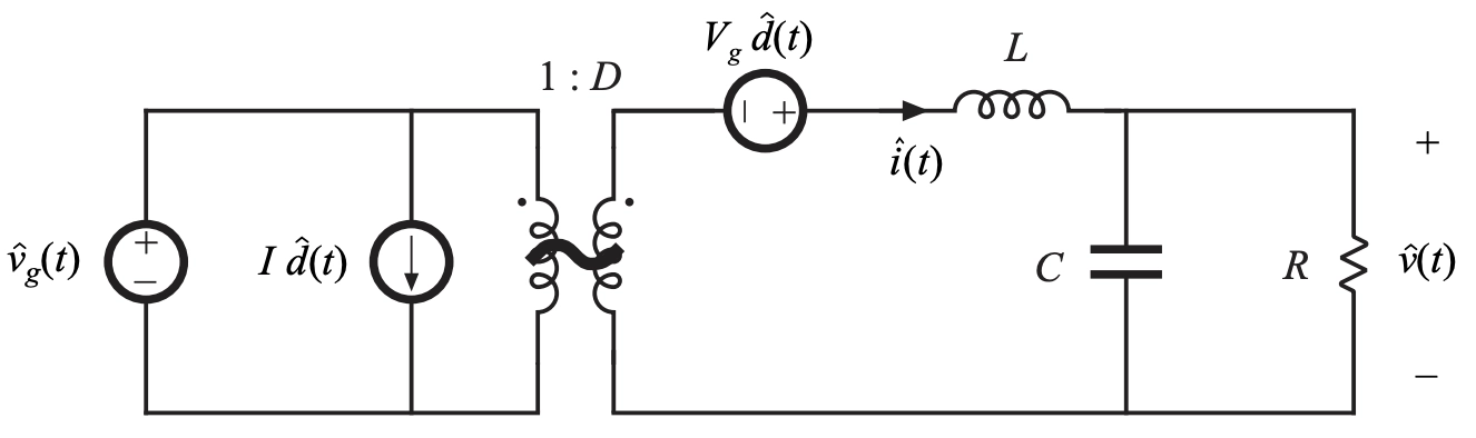
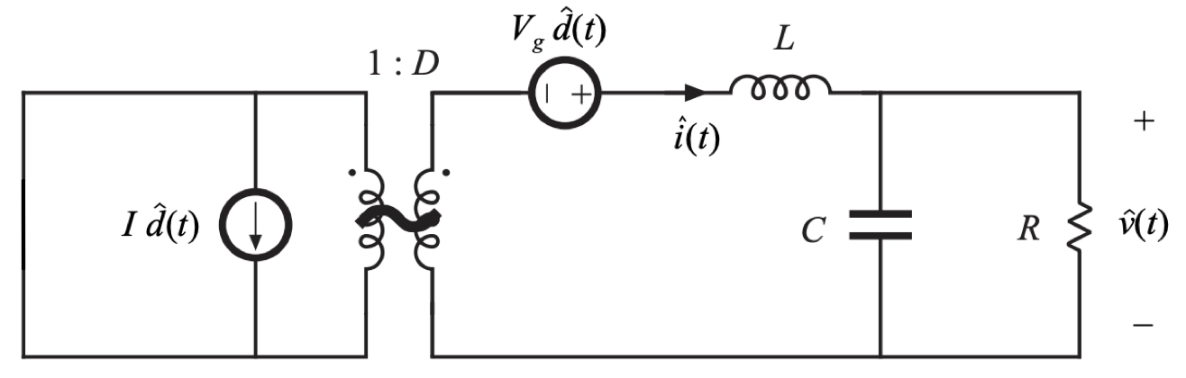
Since we are trying to derive the G_vd, we can assume the small signal perturbation on V_g to be zero. Therefore, Fig. 1 can be simplified as:

Fig. 2Simplified Buck converter small signal model for Gvd derivation^[1]

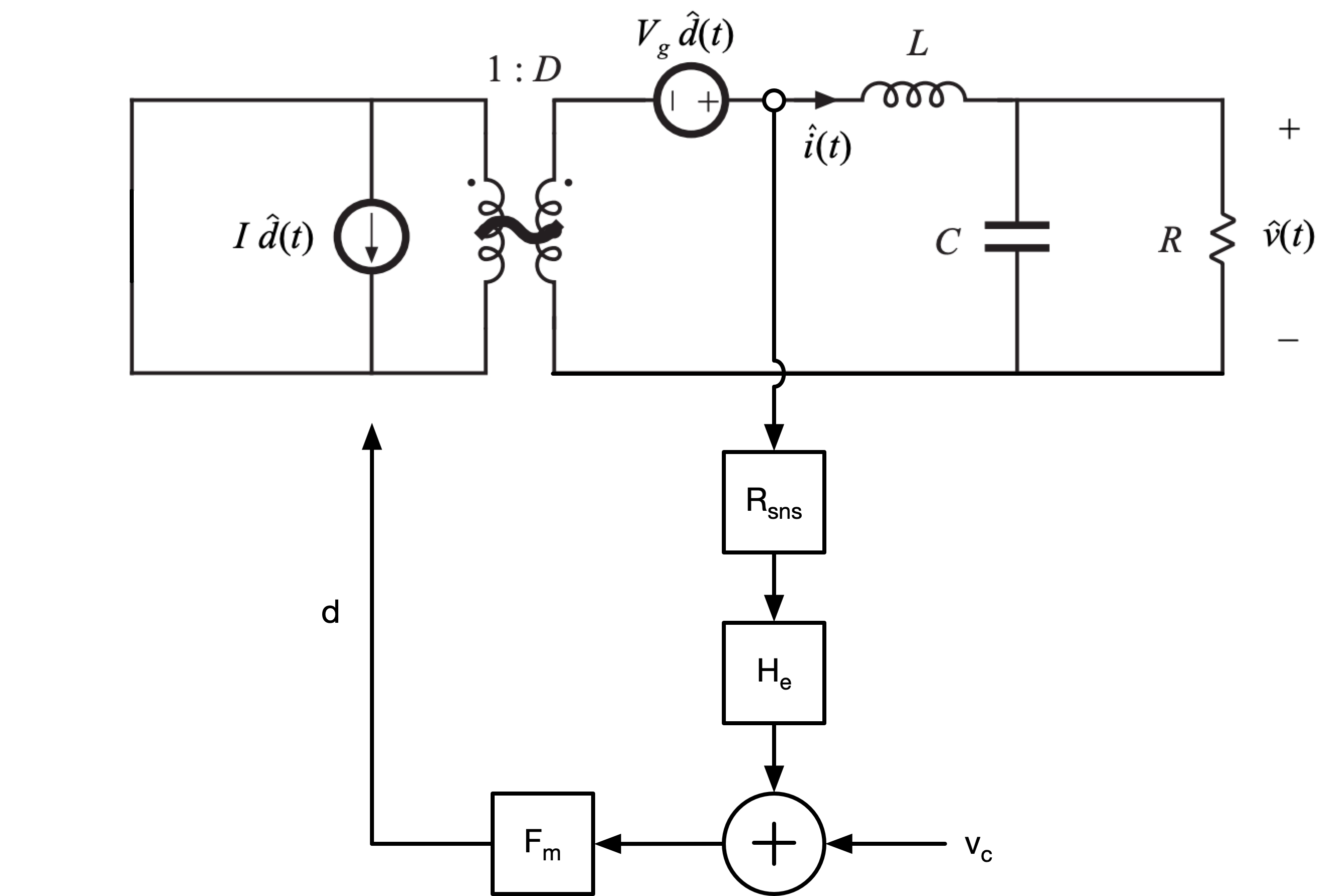
From Fig. 3.4 in Ref. [2], we can draw the current mode controlled Buck converter small signal model as shown in Fig. 3, where:

• R_sns is the current sense gain
• H_e is the transfer function for describing the subharmonic pole effect
• F_m is the modulator gain

Fig. 3Current mode controlled Buck converter small signal model^[2]

Step 1 - depict the transient waveform in time domain

The transient waveform is shown in Fig. 4, where we assume a small perturbation i_L[k] happened on the inductor current. By using the waveform in the time domain, we can calculate the perturbation of the inductor current in the next cycle.

Fig. 4Time domain waveforms for peak current mode controlled Buck converter

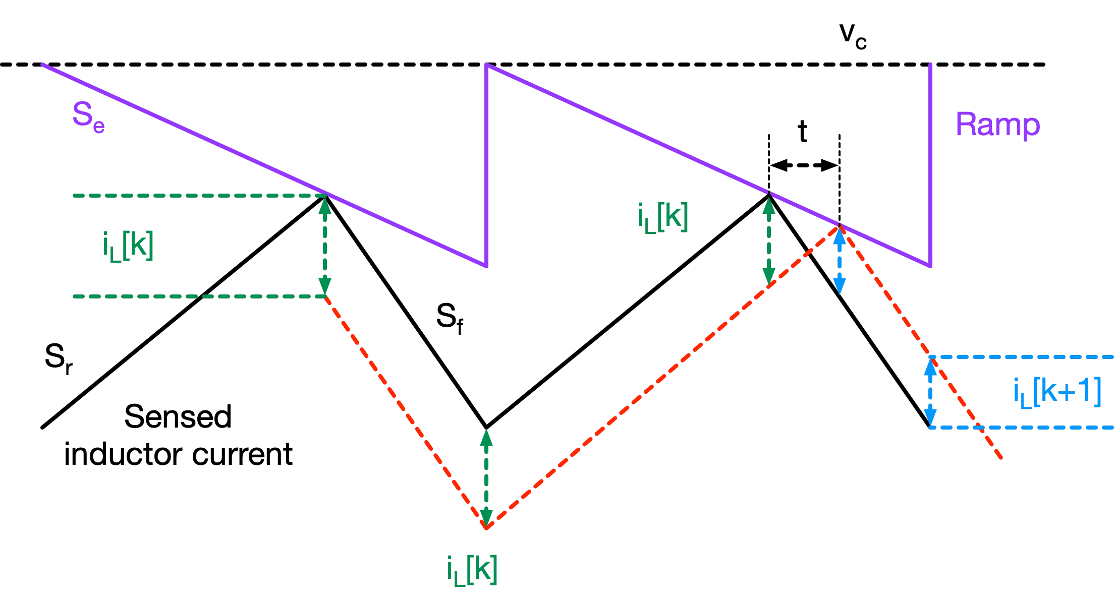
Fig. 5 shows a zoom-in portion of Fig. 4, which can be used for calculating the perturbation.

Fig. 5Time domain waveforms for peak current mode controlled Buck converter - zoom in

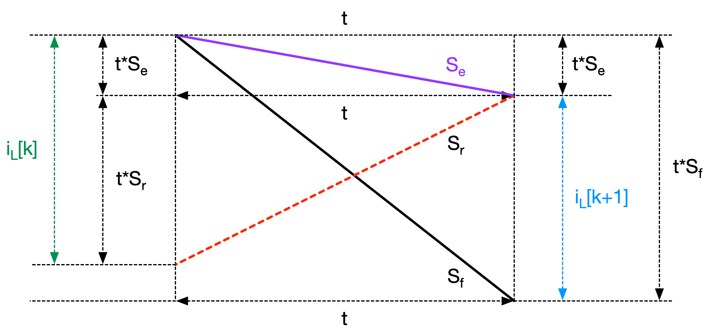
For i_L[k], it is a negative number since the perturbation is negative. From Fig. 5, we have:

For i_L[k+1], it is a positive number since the inductor current is increasing at [k+1] time period. From Fig. 5, we have:

By combining Eq. 1~2, we have:

From Eq. 3, we know that:

• If we do not have the compensation ramp (meaning S_e is equal to 0), i_L[k+1] will start to increase when S_f is greater than S_e, which means duty cycle is greater than 50%. To summarize, when there is no compensation ramp, subharmonic oscillation will start to appear when the duty cycle is greater than 50%.
• If the compensation ramp slope S_e tracks inductor current down slope (S_e = S_f)

Next, we can set:

Therefore, Eq. 3 can be rewritten as:

Step 2 - VEA perturbation

In Step 1, we have calculated the perturbation of the inductor current and how it propagates in the next cycle. Now let us calculate the perturbation of EA (error amplifier). The perturbation of V_c or V_EA is as shown in Fig. 6.

Fig. 6VEA perturbation to the inductor current

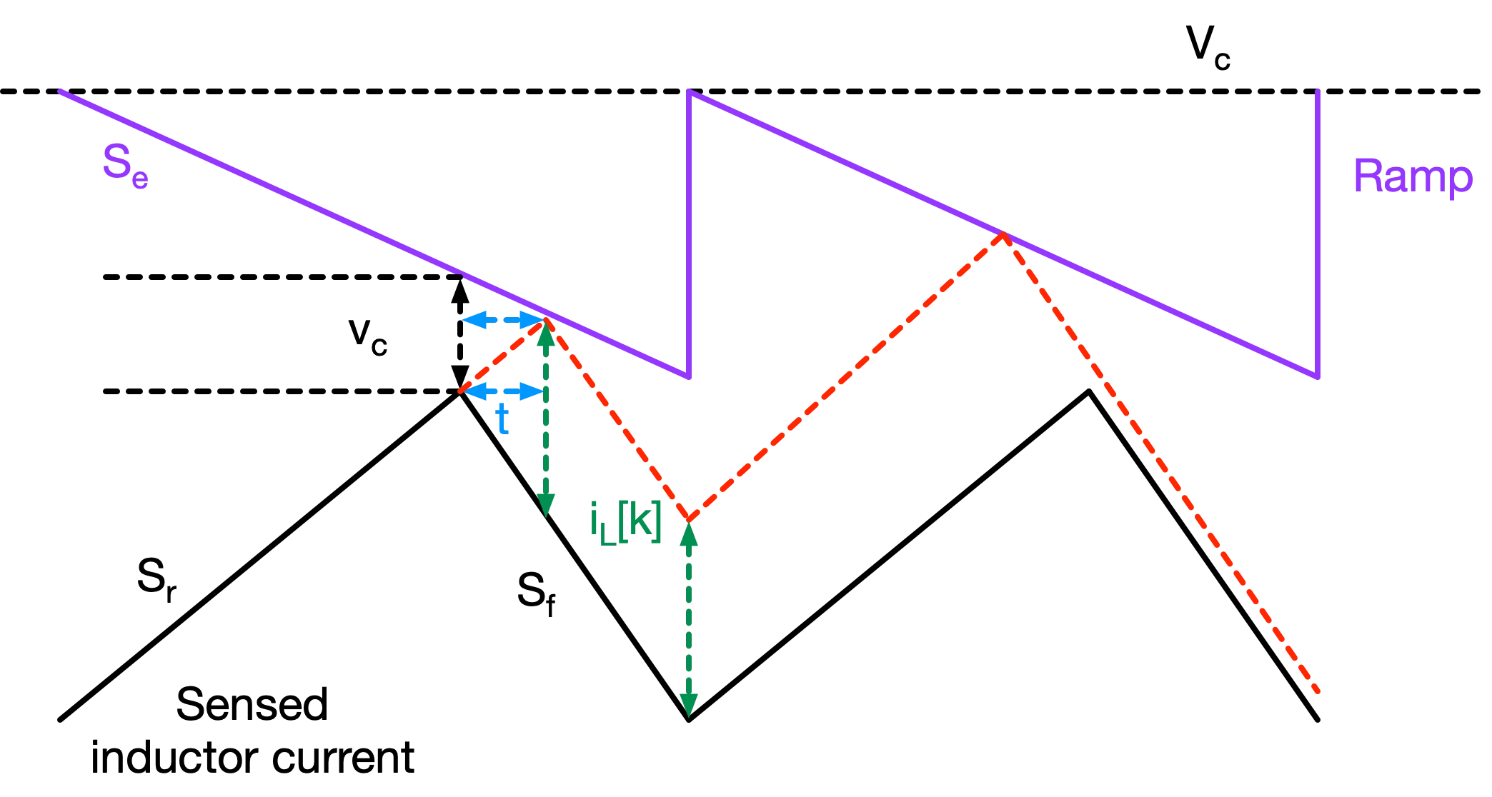
From Fig. 6, we have:

We also know that:

By combining Eq. 6~7, we have:

Therefore,

By combing Eq. 4 and Eq. 9, we have:

Or,

By combing Eq. 5 and Eq. 11, through superposition, we have:

Step 3 - z-domain transfer function

Eq. 12 gives a time domain discrete transfer function which can be easily traferred into the z-domain. We have:

Eq. 13 can be factored as:

Therefore, we have:

s-domain transfer function

Next, let us change the z domain transfer function Eq. 15 to the s domain transfer function using the following method:

Therefore, Eq. 15 can be mapped into the s domain as:

Eq. 16 can be re-written as:

Step 4 - H(s) derivation based on Fig. 3

The modulator gain F_m can be written as:

Here we are trying to calculate the subharmic pole. Therefore, we can assume the input and output is constant. Therefore, Buck converter output is AC ground. As a result, Fig. 3 can be further simplified as shown in Fig. 7.

Fig. 7Current mode controlled Buck converter small signal model - VOUT AC grounded

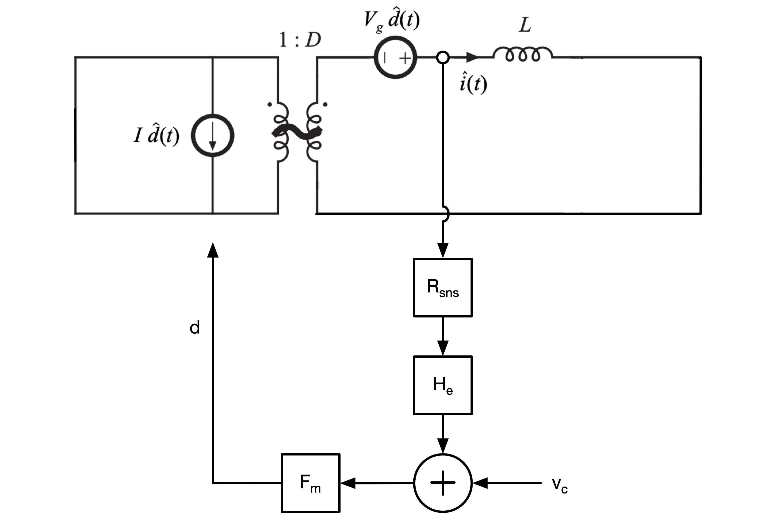
From Fig. 7, we have:

The up slope of sensed inductor current in voltage domain can be calculated as:

The down slope of sensed inductor current in voltage domain can be calculated as:

From Eq. 21~22, we have:

By combing Eq. 20 and Eq. 23, we have:

Therefore,

From Fig. 7, we have:

By comparing Eq. 25~26, we have:

Therefore, we have:

From Eq. 28, we have:

By comparing Eq. 18 and Eq. 29, we have:

We can remove R_sns from both left and right side as:

Eq. 32 can be further simplified as:

By combing Eq. 19 and Eq. 32, we have:

We know that:

Therefore,

Eq. 35 can be re-written as:

Or,

Eq. 37 can be re-written as:

Finally,

Step 5 - simplification of H_e(s)

We can use the complexed pole transfer function to approximate Eq. 39 to get a more simplified equation as:

Where,

And,

The following Matlab script can be used for verification of the simplified equation vs the original transfer function.

clc; clear; close all;

Ts = 1e-6;
wn = pi/Ts;
Q = -2/pi;
s = tf('s');

H1 = exp(-s*Ts)*s*Ts/(1-exp(-s*Ts));
H2 = 1+s/wn/Q + (s/wn)^2;

opts = bodeoptions('cstprefs');
opts.PhaseWrapping='on';
h = bodeplot(H1, opts);  
hold on;
h = bodeplot(H2, opts);
setoptions(h, 'FreqUnits', 'Hz');   % change frequency scale from rad/sec to Hz
set(findall(gcf,'type','line'),'linewidth',2)
grid on;
hold on;
xlim([10, 10e6]);
legend("exponential", "simplified");

The bode plot comparison is as shown in Fig. 8 to prove that Eq. 40 can be used to approximate Eq. 39.

Fig. 8Comparison between the acutual equation and the approximation

We can see that up to half of the switching frequency, the simplifed equation does track the actual transfer function very well.

References and downloads

[1] A New Small-Signal Model for Current-Mode Control

[2] Chapter 7. AC Equivalent Circuit Modeling - slide 41