Monte Carlo simulation in Xschem

Test bench

Fig. 1 shows the test bench of current mirror mismatch^[1]. We use an ideal 1µA current source to bias the current mirror, whose width is 1µm and length is 5µm. For the current mirror device, we use an ideal voltage source to bias its Vds to be 900mV.

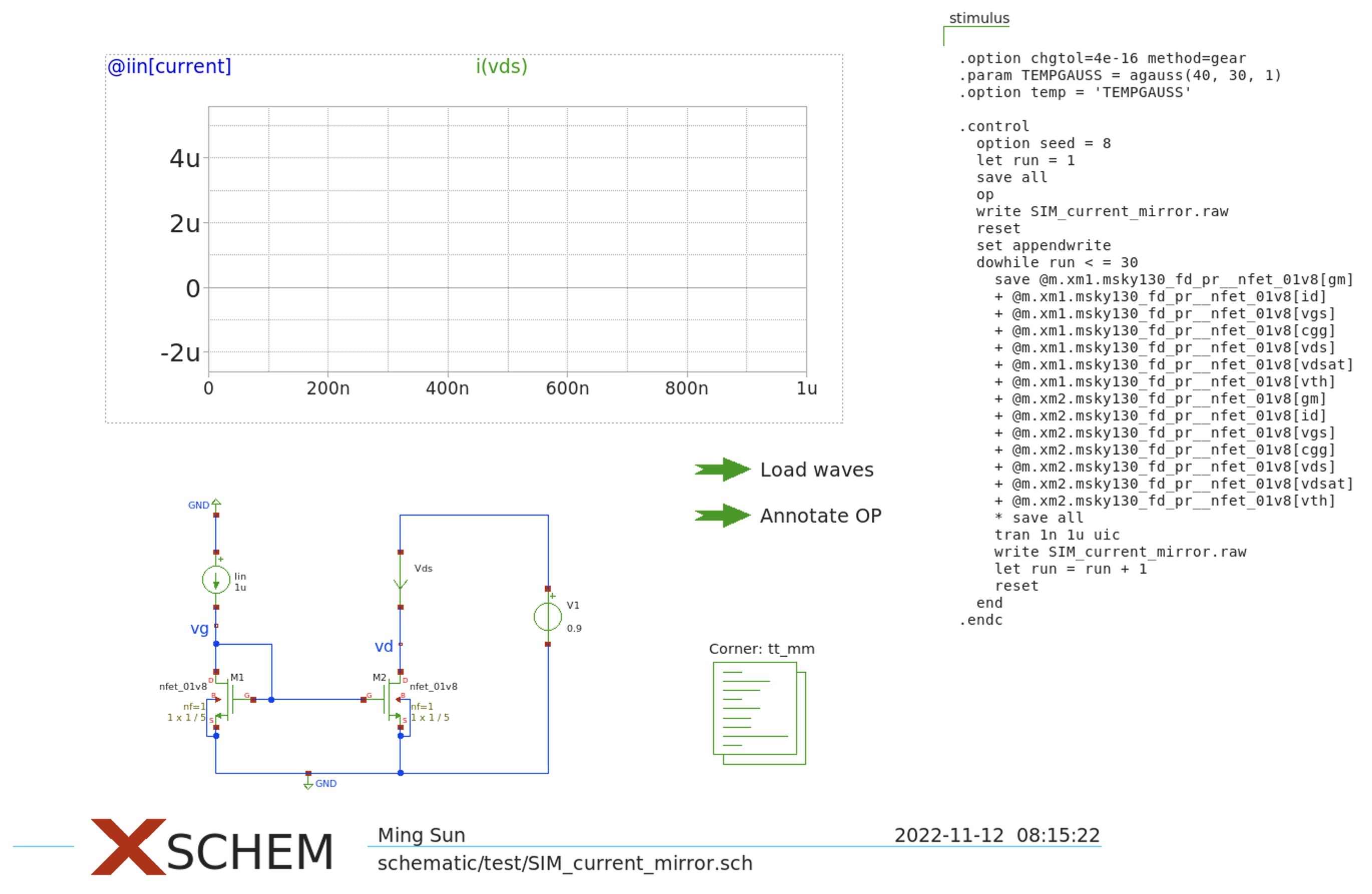
Fig. 1Current mirror test bench for monte carlo simulation

Key components in the test bench

• nfet_01v8 from xschem/sky130_fd_pr
• ammeter.sym from xschem_library/devices
• built-in waveform graph

• corner.sym from xschem/sky130_fd_pr with the following contents. Here we use tt_mm model so that we can include the mismatch information into the monte carlo simulation.

name=CORNER only_toplevel=true corner=tt_mm

• code_shown.sym from xschem_library/devices with the following contents. Basically we are going to run the test bench for 50 runs. For each run, we are going to use the tt_mm mismatch model and vary the temperature settings. As a result, the monte carlo simulation result is going to include the process and temperature variations.

name=stimulus 
only_toplevel=false 
place=end

value="
.option chgtol=4e-16 method=gear
.param TEMPGAUSS = agauss(40, 30, 1)
.option temp = 'TEMPGAUSS'

.control
  option seed = 8
  let run = 1
  save all
  op
  write SIM_current_mirror.raw
  reset
  set appendwrite
  dowhile run < = 50
    save @m.xm1.msky130_fd_pr__nfet_01v8[gm] 
    + @m.xm1.msky130_fd_pr__nfet_01v8[id]
    + @m.xm1.msky130_fd_pr__nfet_01v8[vgs]
    + @m.xm1.msky130_fd_pr__nfet_01v8[cgg]
    + @m.xm1.msky130_fd_pr__nfet_01v8[vds]
    + @m.xm1.msky130_fd_pr__nfet_01v8[vdsat]
    + @m.xm1.msky130_fd_pr__nfet_01v8[vth]
    + @m.xm2.msky130_fd_pr__nfet_01v8[gm] 
    + @m.xm2.msky130_fd_pr__nfet_01v8[id]
    + @m.xm2.msky130_fd_pr__nfet_01v8[vgs]
    + @m.xm2.msky130_fd_pr__nfet_01v8[cgg]
    + @m.xm2.msky130_fd_pr__nfet_01v8[vds]
    + @m.xm2.msky130_fd_pr__nfet_01v8[vdsat]
    + @m.xm2.msky130_fd_pr__nfet_01v8[vth]
    * save all
    tran 1n 1u uic
    write SIM_current_mirror.raw
    let run = run + 1
    reset
  end
.endc
"

• launcher.sym from xschem_library/devices to load/unload the simulation data

name=h17 
descr="Load waves" 
tclcommand="
xschem raw_read $netlist_dir/[file tail [file rootname [xschem get current_name]]].raw tran

"

• launcher.sym from xschem_library/devices to annotate the operating point. Notice that we can also use the live annotation with b cursor as well.

name=h15
descr="Annotate OP" 
tclcommand="set show_hidden_texts 1; xschem annotate_op"

Simulation results

After the simulation is done, we can load the simulation data. The monte carlo simulation result is as shown in Fig. 2.

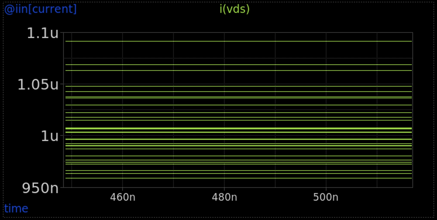
Fig. 2Monte carlo simulation results

From Fig. 2, we can see that the monte carlo simulation does work and the drain current of M2 current mirror varies between 1.1µA and 950nA. To better view the mean and standard deviation, we can use Matlab to plot the histogram as shown in Fig. 3.

Fig. 3Current mirror mismatch deviation in Matlab plot

References and materials

[1] SIM_current_mirror schematic svg

[2] SIM_current_mirror.sch - download