Ming Sun – Silicon achitect, design lead, researcher.

Type-III compensator - OTA based

Fig. 1 shows a Type-III compensator, where an OTA is being used. Different than the Opamp case, Type-III compensator implemented by OTA does not have local feedback loop^[1]. Type-III compensator can be used to boost the phase margin for voltage-mode controlled switching regulators.

Fig. 1Type-III compensator block diagram^[1]

Where,

R1 and R2 is the feedback resistor
R3 and C3 is part of the compensation network of Type-III compensator
Vref is the input referent voltage for EA (error amplifier)
ro is the output impedance of the EA
R4, C4 and C5 is part of the compensation network of Type-III compensator

Fig. 1 can be rearranged to be two groups. One group is the feedback network and another group is the Type-II compensator. Here in the AC analysis, we can assume the contant DC voltage source vref to be AC ground as shown in Fig. 2.

Fig. 2Type-III compensator block diagram - grouped by network^[1]

The transfer function of Type-III compensator is defined as:

`H(s) = (V_(EA))/V_{OUT} = H_1(s)*H_2(s)`

(1)

Feedback network transfer function derivation - H₁(s)

The feedback network transfer function is defined as:

`H_1(s) = (V_(fb))/V_{OUT}`

(2)

The Matlab script used to derive H₁(s) is as shown below.

H1.m

clc; clear; close all;

syms s R1 R2 R3 C3
syms Vout Vfb H1

eqn1 = (Vout-Vfb)/R1 + (Vout-Vfb)/(R3+1/s/C3) == Vfb/R2;
eqn2 = H1 == Vfb/Vout;

results = solve(eqn1,eqn2,[Vfb,H1]);

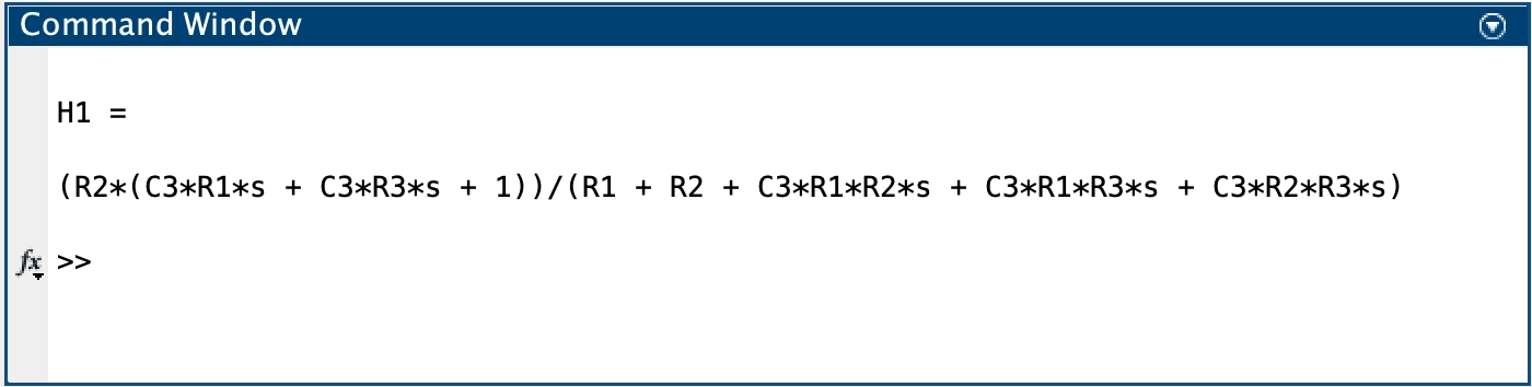
H1 = simplify(results.H1)

The derived result of H₁(s) is as shown in Fig. 3.

Fig. 3H1(s) derivied result from Matlab

Next, we can use wxMaxima to simplify the result as shown in Fig. 4.

Fig. 4H1(s) simplified result from wxMaxima

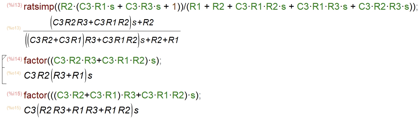
From Fig. 4, we have:

`H_1(s) = (R_2+R_2C_3(R_1+R_3)s)/(R_1+R_2+C_3(R_1R_2+R_1R_3+R_2R_3)s)`

(3)

As a designer, we have the freedom to choose the resistor and capacitor values for Eq. 3. Here we can choose a value so that:

`R_1 text(>>) R_3, R_2 text(>>) R_3`

(4)

Therefore, Eq. 3 can be simplified as:

`H_1(s) = (R_2+R_2C_3R_1s)/(R_1+R_2+C_3R_1R_2s)`

(4)

Then we can factor out the DC term as:

`H_1(s) = R_2/(R_1+R_2)*(1+sR_1C_3)/(1+sC_3(R_1R_2)/(R_1+R_2))`

(5)

Or,

`H_1(s) = R_2/(R_1+R_2)*(1+sR_1C_3)/(1+s(R_1||R_2)C_3`

(6)

The pole and zero location can be calculated as:

`{(z=-1text(/)(R_1C_3)),(p=-1text(/)((R_1||R_2)C_3)):}`

(7)

The zero is at lower frequency than the pole frequency. As a result, we can achieve some amount of phase boost by H₁(s). To gain the maximum phase boost, it is preferred that R₁ is chosen to be much greater than R₂. However, there is a drawback. The feedback divider ratio is typically determined by the V_OUT and V_ref. Once V_OUT and V_ref are chosen, we do not really have too much freedom to modify the phase boost here through H₁(s).

The Matlab script used for sweeping capacitor C₃ is as shown below.

C3_sweep.m

clc; clear; close all;

Vout = 1.8;
Vref = 1.2;
Rtot = 1e6;
C3 = [10e-12, 100e-12, 1e-9];

ratio = Vref/Vout;
R2 = Rtot*ratio;
R1 = Rtot*(1-ratio);
Rpar = R1*R2/(R1+R2);

s = tf('s');


for i=1:1:length(C3)
    H1 = R2/(R1+R2)*(1+s*R1*C3(i))/(1+s*Rpar*C3(i));
    h = bodeplot(H1);                    % Plot the Bode plot of H1(s)
    setoptions(h, 'FreqUnits', 'Hz');   % change frequency scale from rad/sec to Hz
    set(findall(gcf,'type','line'),'linewidth',2)
    grid on;
    hold on;
end

legend("C3=10pF","C3=100pF","C3=1nF")

Fig. 5 shows the H₁(s) Bode plot for different C₃.

Fig. 6H1(s) Bode plot from Matlab - C3 sweep

From Fig. 6, we can easily tell that once the feedback resistor ratio is fixed, the amount of phase boost we can achieved for H₁(s) is pretty much fixed. Changing compensation capacitor C₃ value does not change the phase boost amount. Instead, it just changes the maximum phase boost frequency position.

Here let us keep the total output impedance to be constant at 1MΩ and start to sweep the feedback divider ratio. The Matlab script is as shown below.

ratio_sweep.m

clc; clear; close all;

Vout = 1.8;
Vref = 1.2;
Rtot = 1e6;
C3 = 10e-12;

ratio = [0.5,1,2,5,10];


s = tf('s');


for i=1:1:length(ratio)
    R2 = Rtot*ratio(i);
    R1 = Rtot*(1-ratio(i));
    Rpar = R1*R2/(R1+R2);
    H1 = R2/(R1+R2)*(1+s*R1*C3)/(1+s*Rpar*C3);
    h = bodeplot(H1);                    % Plot the Bode plot of H1(s)
    setoptions(h, 'FreqUnits', 'Hz');   % change frequency scale from rad/sec to Hz
    set(findall(gcf,'type','line'),'linewidth',2)
    grid on;
    hold on;
end

legend("ratio=0.5","ratio=1","ratio=2","ratio=5","ratio=10");

Fig. 7 shows the H₁(s) Bode plot sweep for different feedback ratio.

Fig. 7H1(s) Bode plot from Matlab - ratio sweep

OTA based the Type-III compensator is not widely used in the industry. This is because the AC and DC transfer functions are coupled with each other and we do not have too much feedom to achieve the phase boost we desired.

Type-III compensator - Opamp based

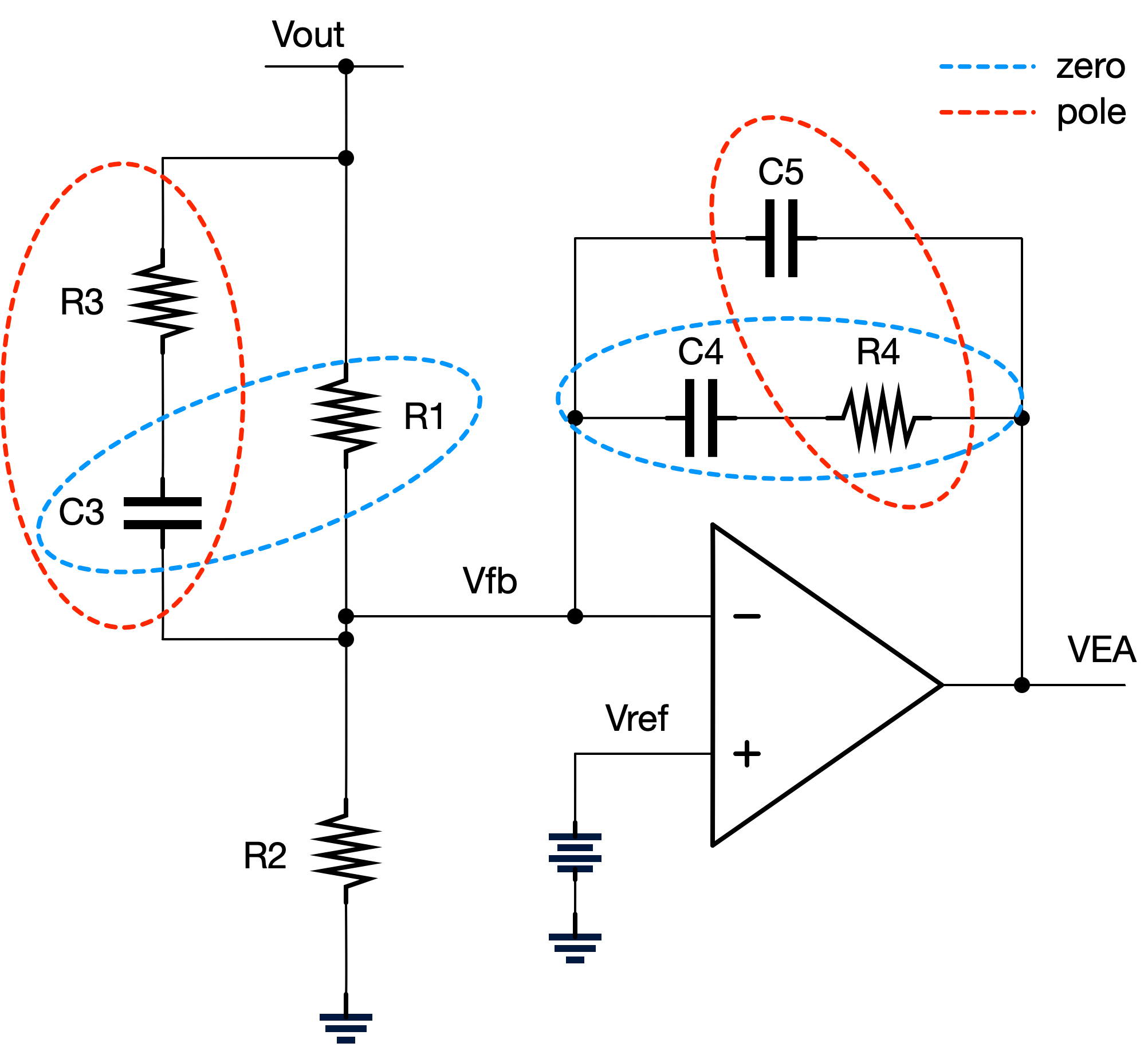
The Opamp based Type-III compensator is as shown in Fig. 8.

Fig. 8Opamp based Type-III compensator

Here we have a local feedback network which is comprised of R₄, C₄ and C₅. Due to the local feedback network, V_fb is virtually connected to V_ref which is AC ground. Therefore, the voltage across resistor R₂ is 0V and there is no AC current flowing through resistor R₂. As a result, resistor R₂ can be considered as an open circuit and can be removed from the small signal model, as shown in Fig. 9.

Fig. 9Opamp based Type-III compensator - small signal model

The following Matlab script can be used to derive the Opamp based Type-III compensator.

type-iii-opamp.m

clc; clear; close all;

syms Vout Vea
syms R1 R3 C3 R4 C4 C5
syms H s

eqn1 = Vout/R1 + Vout/(R3+1/s/C3) + Vea*s*C5 + Vea/(R4+1/s/C4) == 0;
eqn2 = H == Vea/Vout;

results = solve(eqn1,eqn2,[Vea, H]);

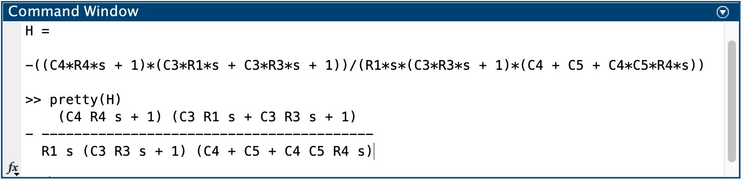
H = simplify(results.H)

The derived transfer function from Matlab is as shown in Fig. 10.

Fig. 10Opamp based Type-III compensator small signal transfer function

Let us make the following assumption to further simplify the transfer function.

`{(R_1text( >> )R_3),(C_4text( >> )C_5):}`

(8)

The simplified transfer function by wxMaxima is as shown in Fig. 11.

Fig. 11Opamp based Type-III compensator small signal transfer function - simplifed

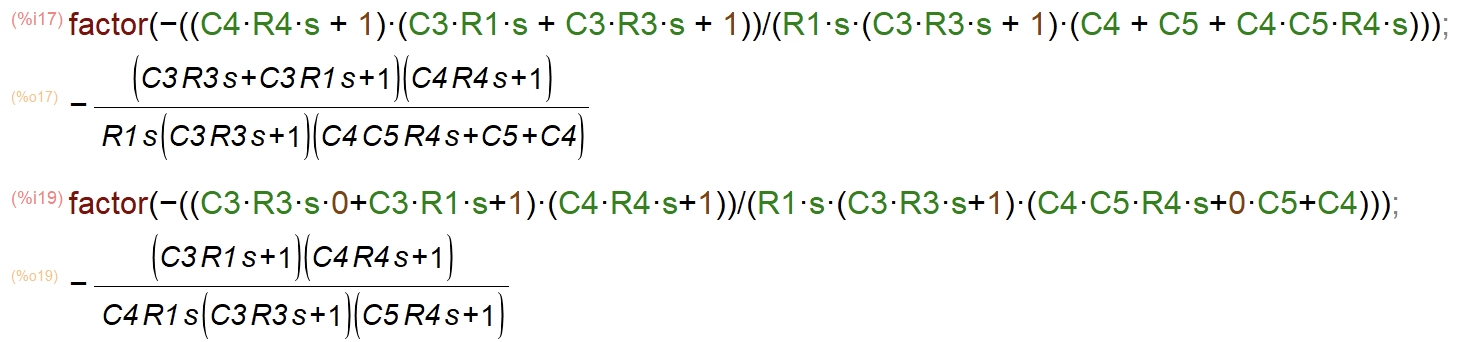
From Fig. 11, we have:

`H=(V_(EA))/(V_(OUT)) = -((1+sR_1C_3)(1+sR_4C_4))/(sR_1C_4(1+sR_3C_3)(1+sR_4C_5))`

(9)

Fig. 12 visually shows the components which generate the poles and zeros in Eq. 9.

Fig. 12Opamp based Type-III compensator - poles and zeros

Next, we can use the following Matlab script to check the Bode plot for the Opamp based Type-III compensator transfer function.

type-III-opamp-based.m

clc; clear; close all;

s = tf('s');

Rtot = 1e6;
Vref = 1.2;
Vout = 1.8;

ratio = Vref/Vout;
R2 = ratio*Rtot;
R1 = (1-ratio)*Rtot;

C3 = 100e-12;
R3 = 1e3;

C4 = 50e-12;
R4 = 500e3;
C5 = 100e-15;

p1 = 1/2/pi/R3/C3;
p2 = 1/2/pi/R4/C5;
z1 = 1/2/pi/R1/C3;
z2 = 1/2/pi/R4/C4;

H = -(1+s*R1*C3)*(1+s*R4*C4)/s/R1/C4/(1+s*R3*C3)/(1+s*R4*C5);

h = bodeplot(H);                    % Plot the Bode plot of H1(s)
setoptions(h, 'FreqUnits', 'Hz');   % change frequency scale from rad/sec to Hz
set(findall(gcf,'type','line'),'linewidth',2)
grid on;
hold on;

ax = findobj(gcf, 'type', 'axes');
phase_ax = ax(1);
mag_ax = ax(2);
xlim([100, 100e6]);
yrange = ylim(mag_ax);

plot(mag_ax, [p1,p1], yrange, ':', 'LineWidth', 2, "Color", "#3B82F6");
plot(mag_ax, [z1,z1], yrange, ':', 'LineWidth', 2, "Color", "#EF4444");
plot(mag_ax, [p2,p2], yrange, '--', 'LineWidth', 2, "Color", "#3B82F6");
plot(mag_ax, [z2,z2], yrange, '--', 'LineWidth', 2, "Color", "#EF4444");

legend(mag_ax, "Bode plot","pole1","zero1","pole2","zero2");

The Bode plot is as shown in Fig. 13.

Fig. 13Opamp based Type-III compensator - Bode plot

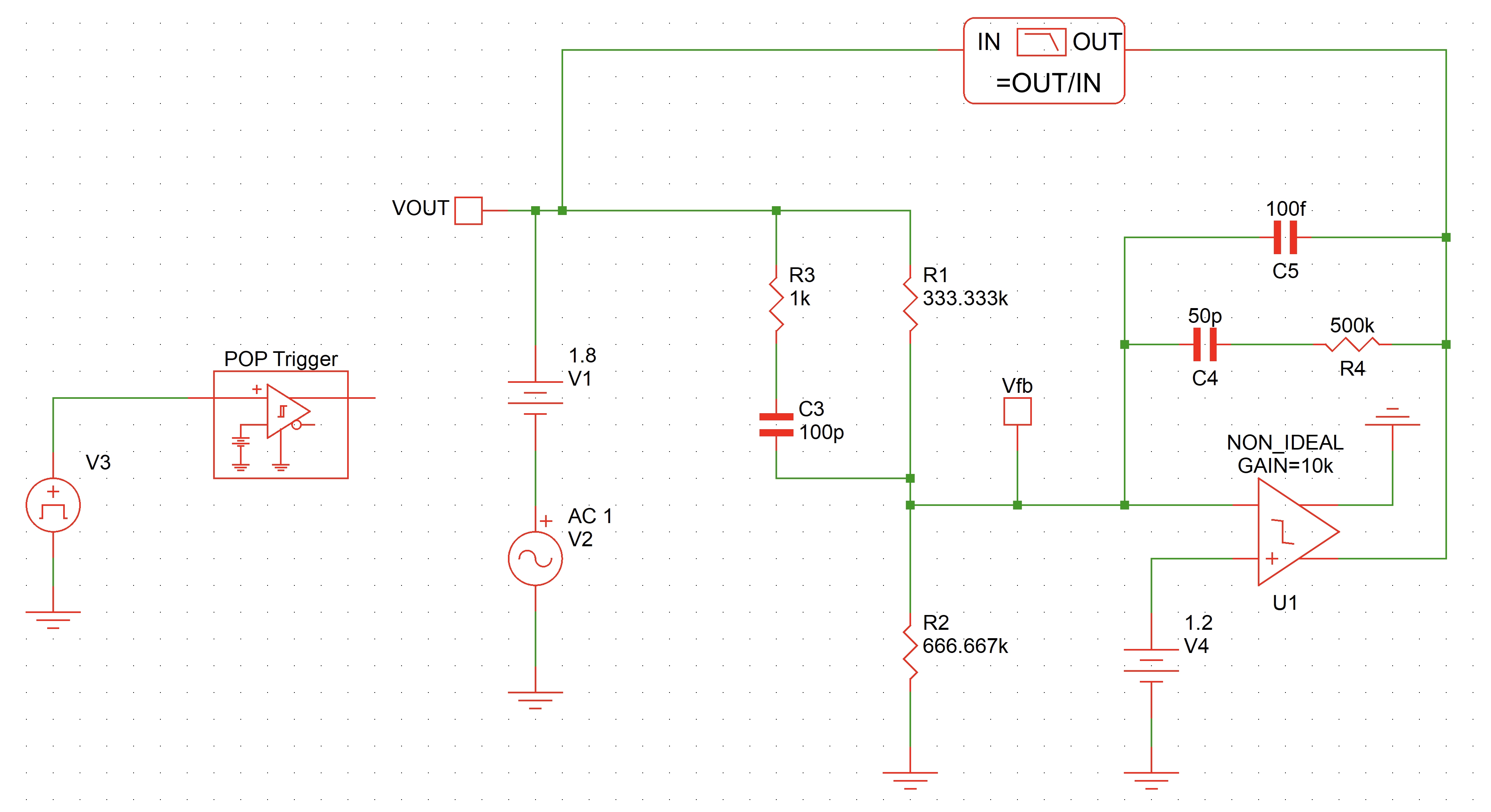
Simplis verification

To verify the Mathematical derivation, the Type-III compensator test bench is created in Simplis as shown in Fig. 14.

Fig. 14Simplis test bench for Opamp based Type-III compensator

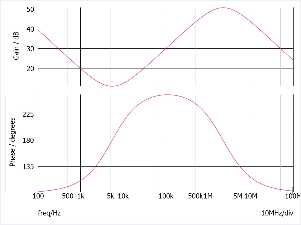
The AC simulation results are as shown in Fig. 15.

Fig. 15AC simulation result of Type-III compensator

Then, we can import the Simplis results into Matlab and compare the Bode plot. The Matlab script is as shown below.

compare.m

clc; clear; close all;

s = tf('s');

Rtot = 1e6;
Vref = 1.2;
Vout = 1.8;

ratio = Vref/Vout;
R2 = ratio*Rtot;
R1 = (1-ratio)*Rtot;

C3 = 100e-12;
R3 = 1e3;

C4 = 50e-12;
R4 = 500e3;
C5 = 100e-15;

p1 = 1/2/pi/R3/C3;
p2 = 1/2/pi/R4/C5;
z1 = 1/2/pi/R1/C3;
z2 = 1/2/pi/R4/C4;

H = -(1+s*R1*C3)*(1+s*R4*C4)/s/R1/C4/(1+s*R3*C3)/(1+s*R4*C5);

h = bodeplot(H);                    % Plot the Bode plot of H1(s)
setoptions(h, 'FreqUnits', 'Hz');   % change frequency scale from rad/sec to Hz
set(findall(gcf,'type','line'),'linewidth',2)
grid on;
hold on;

ax = findobj(gcf, 'type', 'axes');
phase_ax = ax(1);
mag_ax = ax(2);
xlim([100, 100e6]);

% read simplis simulation results from csv file
data = csvread("simplis.csv", 1, 0);
freq_simplis = data(:,1);
mag_simplis = data(:,2);
phase_simplis = data(:,3);

plot(phase_ax, freq_simplis, phase_simplis, 'r--', 'LineWidth', 2);
plot(mag_ax, freq_simplis, mag_simplis, 'r--', 'LineWidth', 2);
legend('Math', 'Simplis')

Fig. 16 shows that the Mathematics derivation perfectly matches with the Simplis AC simulation results.

Conclusion

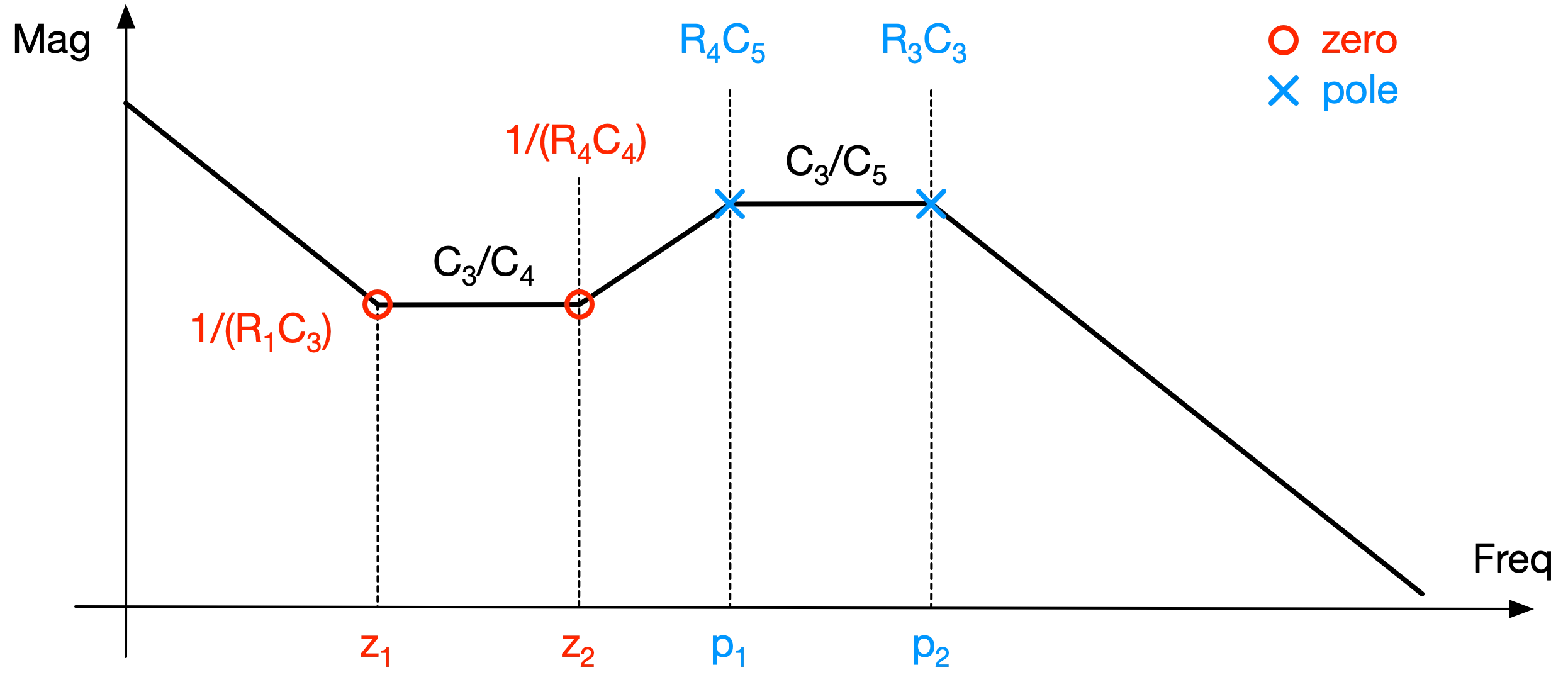
Fig. 17 visually shows the components which generate the poles and zeros in Opamp-based Type-III compensator.

Fig. 17Opamp based Type-III compensator - poles and zeros

There may be different cases for the Bode plot, which is determiend by how we choose the compensation network resistor and capacitor values. The following shows three cases, which demonstrate how the Bode plot midband gain is affected by the poles and zeros.