Ming Sun – Silicon achitect, design lead, researcher.

V_OUT peak to peak ripple calculation

The Buck converter block diagram is as shown in Fig. 1.

Fig. 1Buck power stage block diagram^[1~2]

Fig. 1 shows the inductor current ripple in the time domain. Between t₀ and t₂, the voltage across the inductor is V_IN-V_OUT. As a result, the inductor current slope is positive and inductor current is increasing. Between t₂ and t₄, the voltage across the inductor is -V_OUT. As a result, the inductor current slope is negative and inductor current is decreasing.

Fig. 2Inductor current ripple

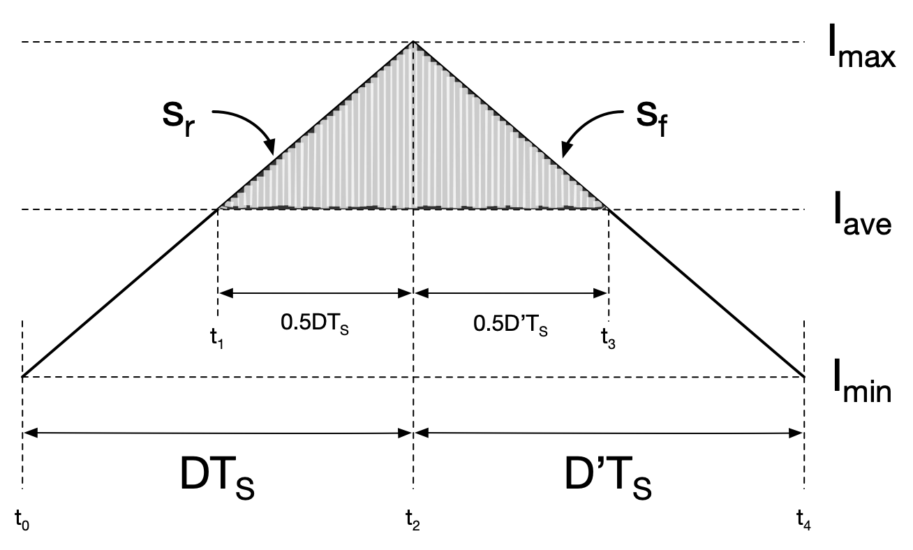
The inductor average current can be calculated as:

`I_{L, ave} = I_R = V_{OUT}/R`

(1)

The inductor current up slope can be calculated as:

`S_{r} = (V_{IN} - V_{OUT})/L = V_{OUT}/L*D^'/D`

(2)

By combing Eq. 1~2 and Fig. 2, the inductor peak current can be calculated as:

`I_{L,max} = I_{L,ave}+S_r*(DT_S)/2 = V_{OUT}/R*(1+(RD^'T_S)/(2L))`

(3)

The DC component of the inductor current flows into the output resistor R. The AC components of the inductor current flows into the capacitor, which will generate the V_OUT ripple. The AC current flows through the output capacitor C is as shown in Fig. 3.

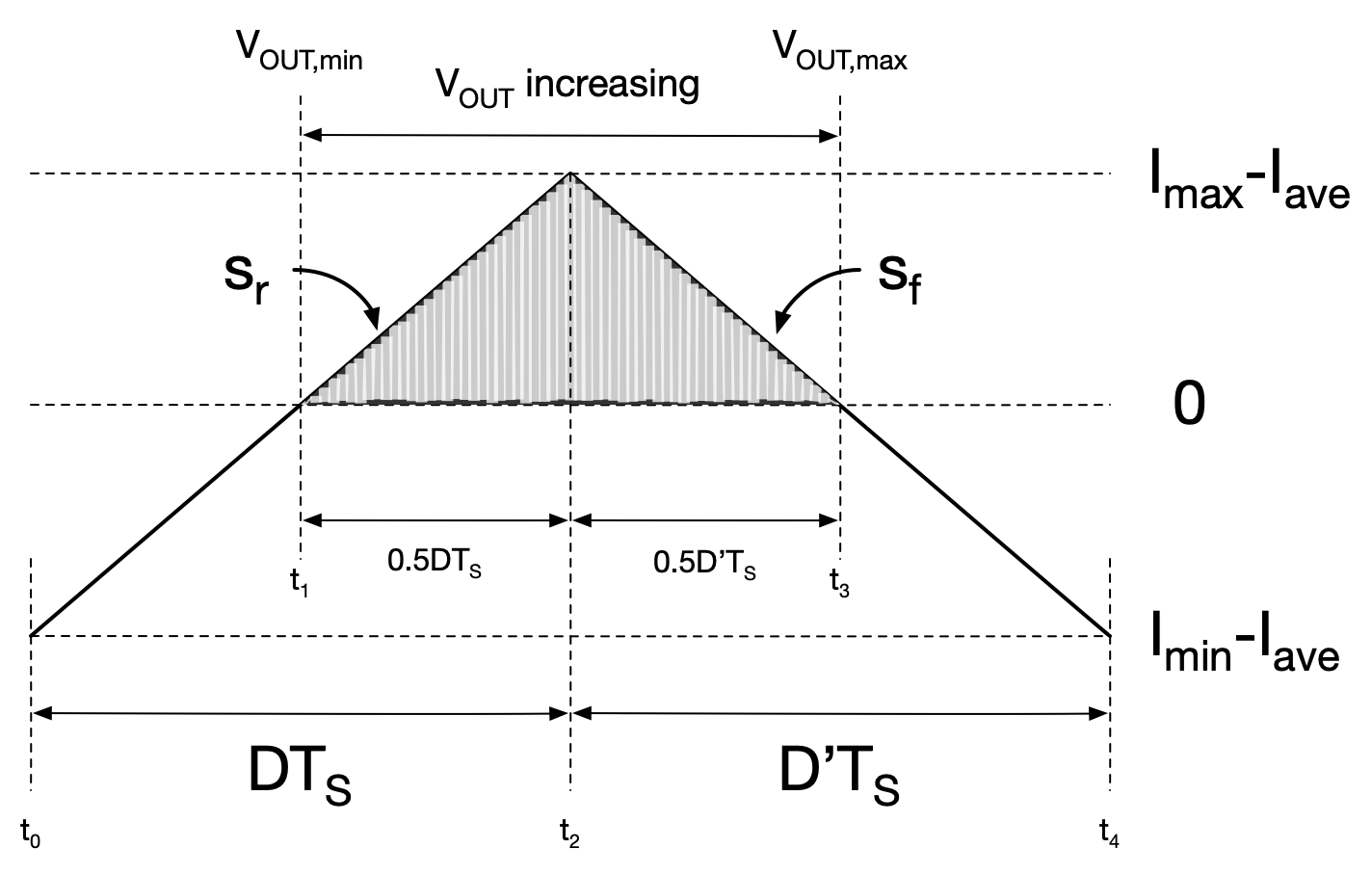
Fig. 3Current flowing through output capacitor

Between t₁ and t₃, there are positive current flowing into the output capacitor C, which will make the output voltage increasing. The output voltage ripple can be calculated as:

`V_{OUT,pp} = 1/C*int_(t_1)^(t_3)Idt = 1/C*1/2*0.5*T_S*(I_{L,max}-I_{L,ave})`

(4)

By combing Eq. 3~4, we have:

`V_{OUT,pp} = 1/(2C)*0.5*T_S*(V_{OUT}D^'T_S)/(2L) = (V_{OUT}D^'T_S^2)/(8LC)`

(5)

Continuous waveform

The current flowing through the capacitor between t₀ and t₂ can be written as:

`I_r(t) = I_{L,min} - I_{L,ave} + S_r*t = -(V_{OUT}*D^'T_S)/(2L) + S_r*t`

(6)

Assuming the output voltage at t₀ is V₀, the capacitor voltage can be calculated as:

`V_{OUT,r}(t) = V_{0} + 1/C*int_(t_0)^(t_2)I_r(t)dt `

(7)

By combining Eq. 6~7, we have:

`V_{OUT,r}(t) = V_{0} - (V_{OUT}*D^'T_S)/(2LC)*t + (S_r*t^2)/(2C)`

(8)

We know that:

`V_{OUT,min}=V_{OUT,r}(t=t_1)=V_{OUT,r}(t=(DT_S)/2)`

(9)

Therefore, the minimum output voltage can be calculated as:

`V_{OUT,min}=V_{0} - (V_{OUT}*DD^'T_S^2)/(8LC) `

(10)

Assume the output voltage at t₂ is V₂. From Eq. 8, we have:

`V_{2}= V_{0} - (V_{OUT}*D^'T_S)/(2LC)*DT_S + (S_r*(DT_S)^2)/(2C) = V_{0}`

(11)

The AC current transfer function between t₂ and t₄ can be written as:

`I_{f}(t) = (V_{OUT}*D^'T_S)/(2L) + S_f*t`

(12)

Where,

`S_f = -V_{OUT}/L`

(13)

The capacitor voltage between t₂ and t₄ can be calculated as:

`V_{OUT,f}(t) = V_{2} + 1/C*int_(t_2)^(t_4)I_{f}(t)dt `

(14)

By combing Eq. 12~14, we have:

`V_{OUT,f}(t) = V_{2} + (V_{OUT}*D^'T_S)/(2LC)*t + (S_f*t^2)/(2C)`

(15)

We know that:

`V_{OUT,max}=V_{OUT,f}(t=t_3)=V_{OUT,f}(t=(D^'T_S)/2)`

(16)

Therefore, the maximum output voltage can be calculated as:

`V_{OUT,max}= V_2 + (V_{OUT}*D^('2)T_S^2)/(8LC) `

(17)

By combing Eq. 11 and Eq.17, we have:

`V_{OUT,max}= V_0 + (V_{OUT}*D^('2)T_S^2)/(8LC) `

(18)

By combing Eq. 10 and Eq.18, we have:

`V_{OUT,pp}= V_{OUT,max}-V_{OUT,min} = (V_{OUT}D^'T_S^2)/(8LC) `

(19)

Eq. 19 matches with Eq. 5 result derived from the charge perspective.

We know that the average voltage of the capacitor should be equal to V_OUT. First, let us integrate the capacitor output between t₀ and t₂ based on Eq. 8. We have:

`int_(t_0)^(t_2)V_{OUT,r}dt = V_0*t - (V_{OUT}*D^'T_S)/(4LC)*t^2 + (S_r*t^3)/(6C)|_{t=DT_S} `

(19)

Eq. 19 can be further simplified as:

`int_(t_0)^(t_2)V_{OUT,r}dt = (DT_S*(12LCV_0 - DD^'T_S^2V_{OUT}))/(12LC) `

(20)

From Eq. 15, we have:

`int_(t_2)^(t_4)V_{OUT,f}dt = V_{0}t + (V_{OUT}*D^'T_S)/(4LC)*t^2 + (S_f*t^3)/(6C)|_(t=D^'T_S)`

(21)

Eq. 21 can be further simplifed as:

`int_(t_2)^(t_4)V_{OUT,f}dt = D^'T_SV_0 + (D^('3)T_S^3)/(12LC)`

(22)

By definition, we have:

`V_{OUT} = (int_(t_0)^(t_2)V_{OUT,r}dt + int_(t_2)^(t_4)V_{OUT,f}dt)/T_S`

(23)

By combining Eq. 20, 22, 23, we have:

`V_{OUT} = V_0 + V_{OUT}*((D^('2)-DD^')T_S^2)/(12LC)`

(24)

Therefore, we have:

`V_{0} = V_{OUT}*[1-((D^('2)-DD^')T_S^2)/(24LC)]`

(25)

Verification

The Matlab script for plotting the inductor current and V_OUT ripple is as shown below.

inductor_current_and_Vout_plot.m

clc; clear; close all;

Vin = 5;
D = 0.5;
L = 1e-6;
C = 1e-6;
R = 1;
Tsw = 1e-6;
Dp = 1 - D;

N = 100;
dt =Tsw/N;

V = D*Vin;
Iave = V/R;
Sr = (Vin-V)/L;
Sf = -V/L;

Imin = Iave - Sr*0.5*D*Tsw;
Imax = Iave + Sr*0.5*D*Tsw;

% V0 = 2.423;
V0 = V*(1-(Dp^2-D*Dp)*Tsw^2/24/L/C);
V2 = V0;
Vo_min = V0 - V*D*Dp*Tsw^2/8/L/C;
Vo_max = V0 + V*Dp^2*Tsw^2/8/L/C;

k=1;
for i=0:dt:D*Tsw
    t(k) = i*1e6;
    I(k) = Imin + Sr*i;
    Vo(k) = V0 - V*Dp*Tsw/2/L/C*i + Sr*i^2/2/C;
    k = k+1;
end

for i=D*Tsw:dt:Tsw
    t(k) = i*1e6;
    I(k) = Imax + Sf*(i-D*Tsw);
    Vo(k) = V2 + V*Dp*Tsw/2/L/C*(i-D*Tsw)+Sf/2/C*(i-D*Tsw)^2;
    k = k+1;
end

for i=Tsw:dt:Tsw+D*Tsw
    t(k) = i*1e6;
    I(k) = Imin + Sr*(i-Tsw);
    Vo(k) = V0 - V*Dp*Tsw/2/L/C*(i-Tsw) + Sr*(i-Tsw)^2/2/C;
    k = k+1;
end

for i=Tsw+D*Tsw:dt:2*Tsw
    t(k) = i*1e6;
    I(k) = Imax + Sf*(i-Tsw-D*Tsw);
    Vo(k) = V2 + V*Dp*Tsw/2/L/C*(i-Tsw-D*Tsw)+Sf/2/C*(i-Tsw-D*Tsw)^2;
    k = k+1;
end

yyaxis('left');
plot(t,I, "LineWidth",2,'Color', '#0284C7');
hold on;
plot([0,2*Tsw*1e6],[Iave,Iave], '--', "LineWidth",1);
% text(0.05e-6, Iave+0.06, '$I_{ave}$ ', 'Interpreter','latex', 'Color', '#0284C7', 'FontSize',16);
plot([D*Tsw*1e6,D*Tsw*1e6],[Imin,Imax], '-.', "LineWidth",1);
plot([Tsw*1e6+D*Tsw*1e6,Tsw*1e6+D*Tsw*1e6],[Imin,Imax], '-.', "LineWidth",1);
% text(0.52e-6, 2.1, '$DT_{S}$ ', 'Interpreter','latex', 'Color', '#0284C7', 'FontSize',16);
plot([0.5*D*Tsw*1e6,0.5*D*Tsw*1e6],[Imin,Imax], ':', "LineWidth",1);
plot([Tsw*1e6+0.5*D*Tsw*1e6,Tsw*1e6+0.5*D*Tsw*1e6],[Imin,Imax], ':', "LineWidth",1);
% text(0.26e-6, 2.1, '$\frac{DT_S}{2}$ ', 'Interpreter','latex', 'Color', '#0284C7', 'FontSize',20);
plot([D*Tsw*1e6+0.5*Dp*Tsw*1e6,D*Tsw*1e6+0.5*Dp*Tsw*1e6],[Imin,Imax], ':', "LineWidth",1);
plot([Tsw*1e6+D*Tsw*1e6+0.5*Dp*Tsw*1e6,Tsw*1e6+D*Tsw*1e6+0.5*Dp*Tsw*1e6],[Imin,Imax], ':', "LineWidth",1);
grid on;
ylim([Imin, Imax]);
ylabel("Inductor current [A]");

yyaxis('right');
plot(t,Vo, "LineWidth",2);
grid on;
ylim([Vo_min, Vo_max]);
ylabel("Output voltage [V]");

xlabel('Time [µs]')

The Matlab plot for duty cycle of 50% is as shown in Fig. 4.

Fig. 4Inductor current and Vout plot - D=50%

The Matlab plot for duty cycle of 50% is as shown in Fig. 5.

Fig. 5Inductor current and Vout plot - D=20%

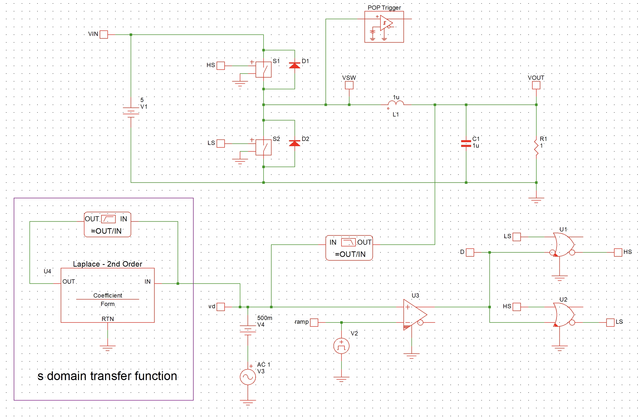
To verify the results and math derivation above, let us build a Buck converter test bench in Simplis as shown in Fig. 6.

Fig. 6Buck converter test bench in Simplis

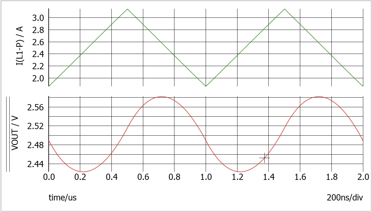
The simulation results from Simplis are as shown in Fig. 7.

Fig. 7Inductor current and output voltage plot from Simplis

We can copy the data from Simplis into csv file and use Matlab to compare the results, which is as shown in Fig. 8.

Fig. 8Inductor current and output voltage comparison betweem Simplis and Math derivations - D=50%

The inductor current matches very well between Simplis simulation results and the Math derivations, while the inductor current shows some mismatches between the two.

References and downloads

[1] Fundamentals of power electronics - Chapter 2

[3] Matlab script for comparison inductor current and output ripple

[4] Simplis test bench

Calculate Vout ripple for Buck converter

VOUT peak to peak ripple calculation

Continuous waveform

Verification

References and downloads

V_OUT peak to peak ripple calculation