Conversion ratio derivation for DCM - Buck converter

Buck converter

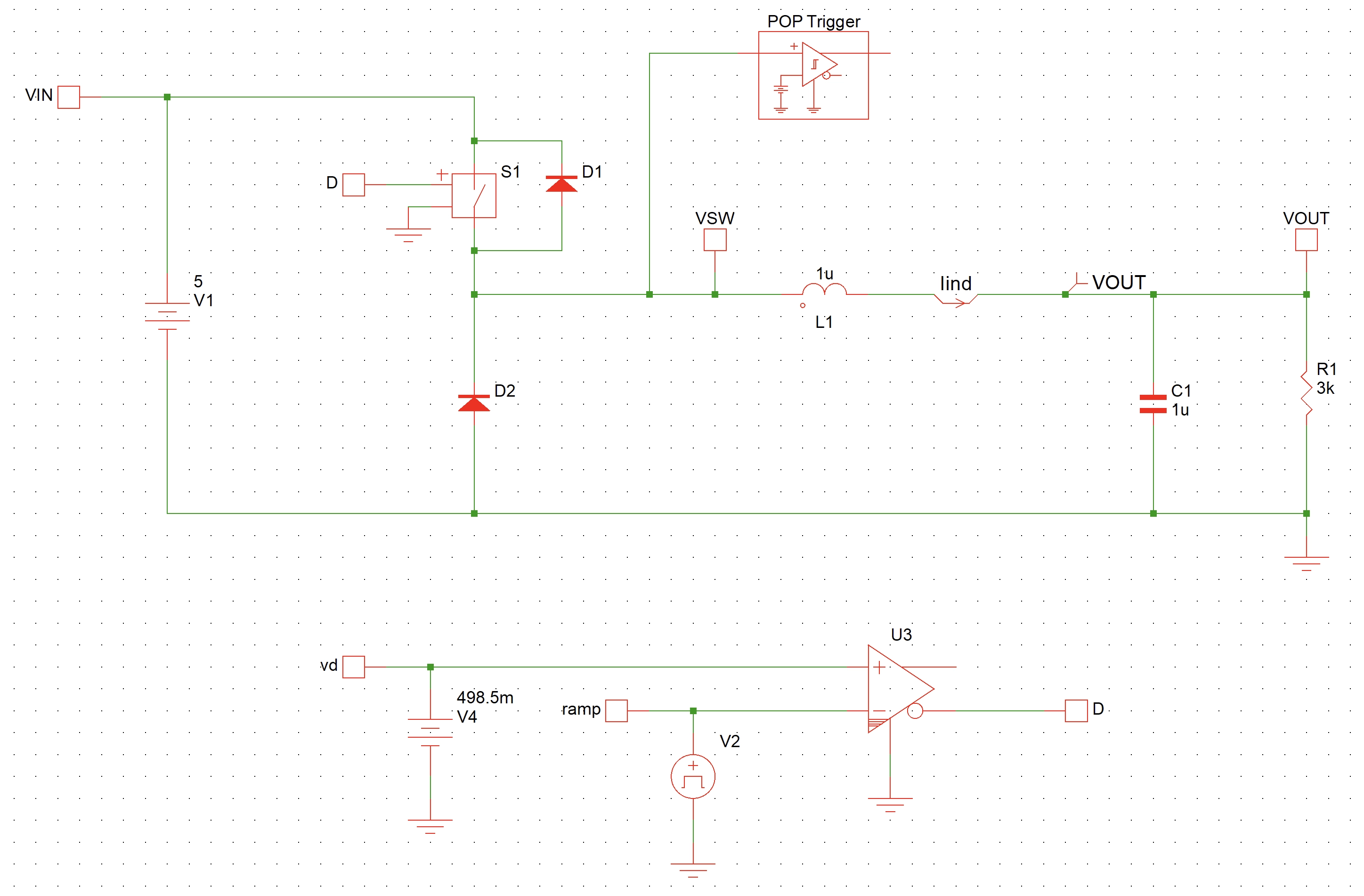
Fig. 1 shows a simple Buck power stage, where a V_IN is the input voltage and V_OUT is the output voltage of the Buck converter^[2].

Fig. 1Asynchronous Buck converter block diagram^[1]

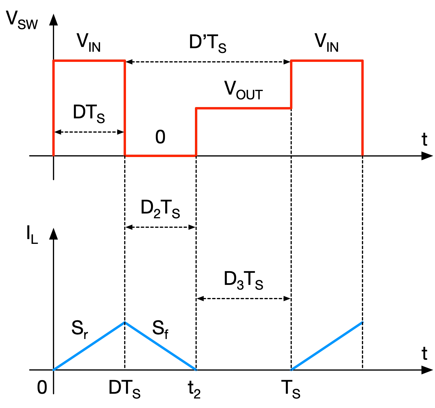
During the light load condition, the converter will automatically enter into the DCM (discontinuous mode) due to the diode D₁. The waveform is as shown in Fig. 2.

Fig. 2Asynchronous Buck converter VSW and inductor current waveform^[1]

Now let us calculate the boundary condition between CCM and DCM. In other words, D₃=0. The Matlab script is as shown below:

clc; clear; close all;

syms D Ts Vg V R Dp L
syms Sr Sf Ipk

eqn1 = D+Dp == 1;
eqn2 = D*(Vg-V) == V*Dp;
eqn3 = Ipk == D*Ts*(Vg-V)/L;
eqn4 = 1/2*Ipk == V/R;

results = solve(eqn1,eqn2,eqn3,eqn4,Dp,Ipk,V, R);

R = simplify(results.R)

The Matlab derived result is as shown in Fig. 3.

Fig. 3Boundary condition between CCM and DCM for Buck converter

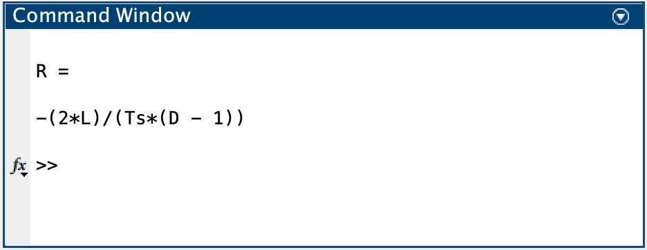
From Fig. 3, we have:

Basically when the load impedance of the Buck converter is greater than R_bound, the converter will enter into DCM operation.

Now, let us derive the conversion ratio M for Buck converter. The Matlab script is as shown below.

clc; clear; close all;

syms D Ts Vg V R D2 D3 Dp L
syms Sr Sf Ipk M

eqn1 = D+D2+D3 == 1;
eqn2 = D*(Vg-V) == V*D2;
eqn3 = Ipk == D*Ts*(Vg-V)/L;
eqn4 = 1/2*(D+D2)*Ipk == V/R;
eqn5 = M == V/Vg;

results = solve(eqn1,eqn2,eqn3,eqn4,eqn5,D2,D3,Ipk,V,M);

M = simplify(results.M)

The Matlab derived result is as shown in Fig. 4.

Fig. 4DCM conversion ratio derivation for Buck converter

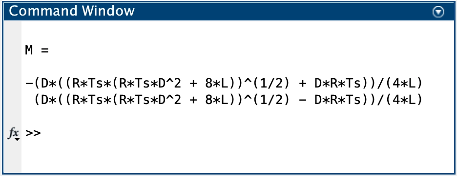
We see there are two derived results from Matlab. We need to figure out which equation is the correct answer. The wxMaxima derived result is as shown in Fig. 5.

Fig. 5DCM conversion ratio simplified results from wxMaxima

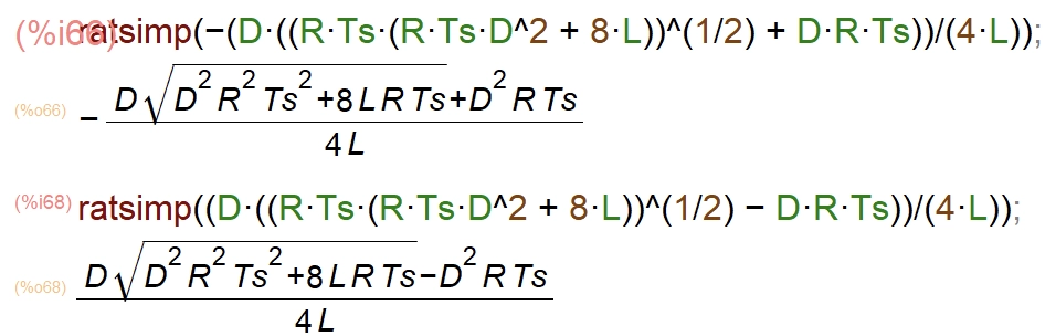
Notice that one of the equations always give a negative conversion ratio, which is not correct. Therefore, we can ignore that equation and the converter ratio can be written as:

Eq. 2 shows the conversion ratio in DCM. Ideally when the load impedance is at R_bound, Eq. 2 should be equal to the CCM conversion ratio D. To verify, the wxMaxima is used to prove this assumption as shown in Fig. 6.

Fig. 6DCM conversion ratio simplification at DCM/CCM boundary condition using wxMaxima

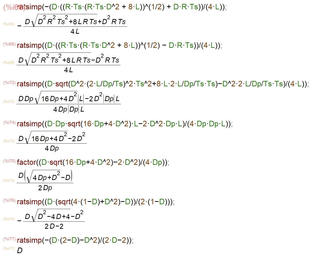
From Fig. 6, we can see that Eq. 2 becomes to the duty cycle D at the boundary condition, which is as we expected.

Next, let us further simplify Eq. 2.

Or,

Therefore, we have:

Where,

Looking at Eq. 1, we know that Eq. 5~6 is only valid when Buck is in DCM. Therefore, we have:

In other words,

Conversion ratio plot

To verify the above Math derivation, the asynchronous Buck converter test bench in Simplis is as shown in Fig. 7.

Fig. 7Asynchronous Buck converter test bench in Simplis

Next, we can set the R1 to different value and compare the Simplis simulation results with Math derivation equations. The Matlab script is as shown below.

clc; clear; close all;

R = linspace(1, 10e3, 10e3+1);

Vg=5;
D=0.5;
L=1e-6;
fsw=1e6;

Ts = 1/fsw;
Dp = 1-D;

for i=1:1:length(R)
    M_dcm(i) = (D*sqrt(D^2*R(i)^2*Ts^2+8*L*R(i)*Ts)-D^2*R(i)*Ts)/4/L;
    M_ccm(i) = D;
end



semilogx(R, M_dcm, 'LineWidth', 2);
hold on;
semilogx(R,M_ccm, 'LineWidth', 2);
grid on;
xlabel('Output impedance [Ω]');
ylabel('conversion ratio')

% simplis data
R_simplis = [1,2,3,5 10,20,30, 100,300, 1e3,3e3, 10e3];
Vout_simplis = [2.4995, 2.5007501,2.5011668,2.7093242,...
    3.3026363,3.8474442,4.1187336, 4.6607649,4.8761196,...
    4.9615067, 4.9870326,4.9960927];

semilogx(R_simplis, Vout_simplis/Vg, 'x',"Color", "#9333EA", "LineWidth", 2, "MarkerSize",12);
legend("DCM equation", "CCM equation", "Simplis", "Location","southeast");

The comparison between Mathematics derivation and Simplis simulation results for conversion ratio is as shown in Fig. 8.

Fig. 8Conversion ratio comparison between Simplis and Math derivation

Conclusion - conversion ratio

Fig. 8 tells us the conversion ratio is simply the maximum between the DCM and CCM Math equation. Then we can combine the conversion ratio equation for DCM and CCM as:

If,

Then, the converter works in CCM. Otherwise, it works in DCM.

References and downloads

[1] Fundamentals of power electronics - Chapter 2

[2] Popular converters and the conversion ratio derivation

[3] Finding the Conversion Ratio M(D,K)

[4] Open-loop asynchronous Buck converter model in Simplis - download