Gvc simulation for peak current mode controlled Boost converter in Simplis

G_vc transfer function for PCM (peak current mode) Boost converter

In Ref. [1], we have derived the G_vc transfer function for PCM controlled Boost converter.

Where, the DC gain is:

The dominant pole is:

The subhamonic oscillation pole is:

The quality factor Q is:

The right half plane zero is:

In this tutorial, let us create the G_vc test bench in Simplis and verify the above equations.

G_vc test bench in Simplis for PCM Boost converter

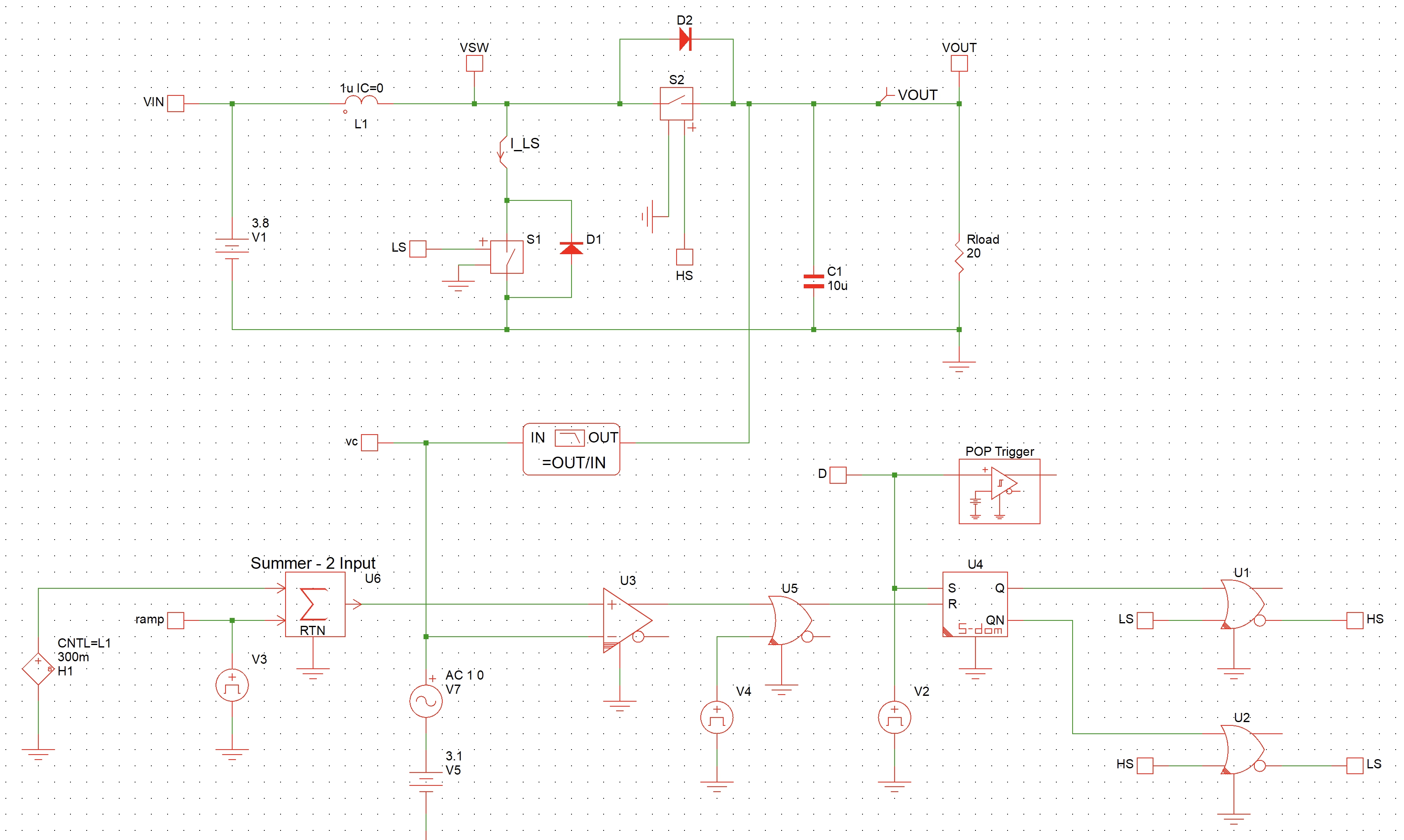
The PCM controlled Boost converter is as shown in Fig. 1.

Fig. 1Gvc test bench for PCM controlled Boost converter in Simplis

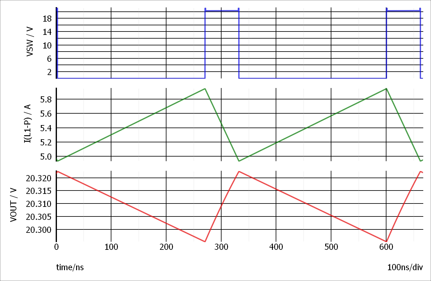
The transient waveforms from Simplis simulation are as shown in Fig. 2.

Fig. 2Transient simulation waveforms from Simplis test bench

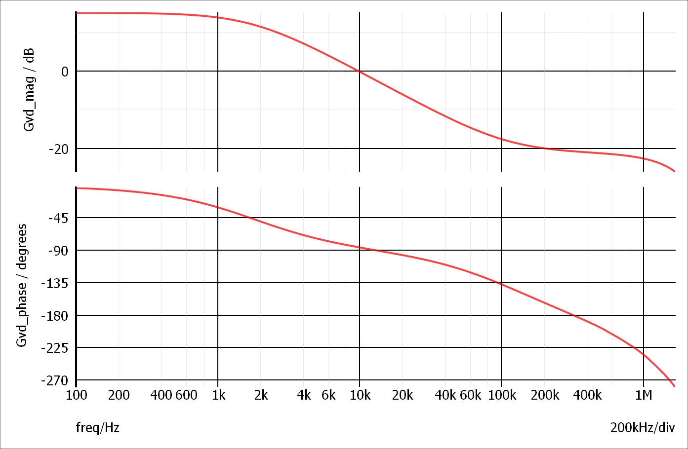
The AC simulation result of G_vc is as shown in Fig. 3.

Fig. 3AC simulation result of Gvc from Simplis

Comparison between Matlab and Simplis

The following Matlab script can be used to compare the G_vc transfer function between Matlab and Simplis.

clc; clear; close all;

Vg = 3.8;
V = 20;
L = 1e-6;
C = 10e-6;
fsw = 3e6;
Rsns = 0.3;
R = 20;

Dp = Vg/V;
D = 1-Dp;
Ts = 1/fsw;
Se = (V-Vg)/L*Rsns;
Sr = Vg/L*Rsns;

s = tf('s');

Gvc0 = R*Dp/(2*Rsns + Dp^3*R*Se*Ts/Vg);
wp = 2/R/C;
wn = pi*fsw;
Q = 1/pi/(Dp*(1+Se/Sr)-0.5);
wrhpz = R*Dp^2/L;

Gvc = Gvc0*(1-s/wrhpz)/(1+s/wp)/(1+s/wn/Q+s^2/wn^2);

h = bodeplot(Gvc);                    % Plot the Bode plot of G(s)
setoptions(h, 'FreqUnits', 'Hz');   % change frequency scale from rad/sec to Hz
set(findall(gcf,'type','line'),'linewidth',2);
p = getoptions(h);
p.PhaseMatching = 'on';
p.PhaseMatchingFreq = 1;
p.PhaseMatchingValue = 0;
setoptions(h,p);

grid on;
hold on;

% read simplis simulation results from csv file
data = csvread("simplis.csv", 1, 0);
freq = data(:,1);
mag = data(:,2);
phase = data(:,3);

ax = findobj(gcf, 'type', 'axes');
phase_ax = ax(1);
mag_ax = ax(2);


% append simplis plot to bode plot
plot(phase_ax, freq, phase, 'r--', 'LineWidth', 2);
plot(mag_ax, freq, mag, 'r--', 'LineWidth', 2);
legend('Math', 'Simplis')
xlim([100, 1.67e6]);

The comparison result from Matlab is as shown in Fig. 4.

Fig. 4Gvc transfer function Bode plot comparison between Mathematics derivation and Simplis

In the above condition, we let compensation ramp to track the inductor current down slope. As a result, Eq. 5 can be written as:

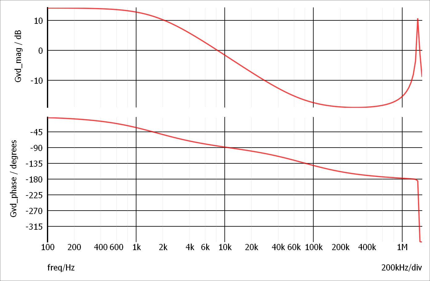
We can run another condition, where we reduce the compensation ramp slope. As a result, the quality factor Q should be increased and we will see higher peaking introduced by the subhamonic poles. The new G_vc plot from AC simulation with reduced compensation ramp slope is as shown in Fig. 5.

Fig. 5Gvc transfer function Bode plot with reduced compensation ramp slope

References and downloads

[1] Modeling of peak current mode controlled Boost converter

[2] Gvc test bench for PCM controlled Boost converter schematic - pdf

[3] Gvc test bench for PCM controlled Boost converter schematic - download