Modeling of peak current mode controlled Boost converter

Boost converter block diagram

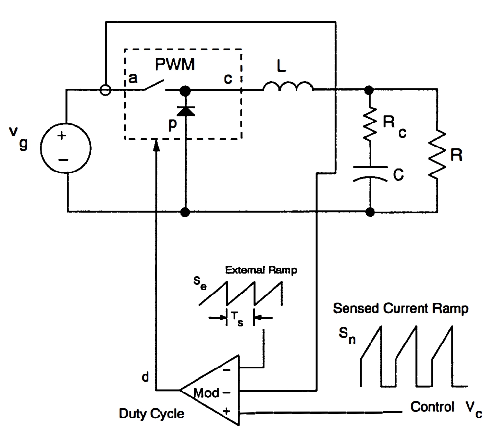
The peak current mode controlled Buck converter is as shown in Fig. 1^[1].

Fig. 1Peak-current mode controlled Buck converter block diagram^[1]

From Fig. 1, we can easily draw the peak current mode controlled Boost converter block diagram as shown in Fig. 2.

Fig. 2Peak-current mode controlled Buck converter block diagram

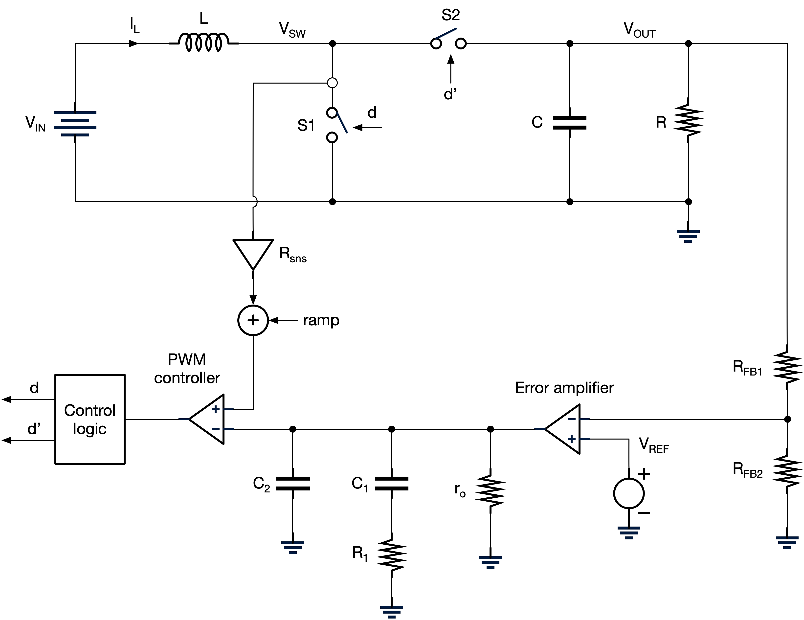
R_FB1 and R_FB2 is the feedback divider. The Error amplifier can be implemented by an OTA, where r_o stands for the output impedance of the OTA. The compensation network is a Type-II compensator, which is comprised of R₁, C₁ and C₂. The biggest advantage of current mode control is that the output complexed poles are gone, which makes the compensation of the converter very easy to be designed.

As the name peak current mode control indicated, the inductor peak current is being sensed through switch S₁. To avoid subharmonic oscillation, a ramp is needed.

Small signal deriviation for G_vc

From inductor voltage second balance equation, we have^[2]:

For the output capacitor charge balance equation, we have^[2]:

G_vc transfer function derivation in Matlab

From Ref. [3], we have derived the transfer function H_e(s), which can be used to mimic the subharmonic pole behavior. We can use H_e(s) in the following Matlab script for peak current mode controlled boost converter G_vc transfer function derivation.

clc; clear; close all;

syms Vg V R C L I
syms Ts
syms D Dp
syms He wn Q
syms s
syms Rsns Sr Se Sf
syms v i d vc 
syms Gvc



eqn1 = s*L*i == -Dp*v + d*V;
eqn2 = s*C*v == Dp*i - d*I - v/R;
eqn3 = He*i*Rsns == vc - Se*d*Ts - Sr*d*Ts;
eqn4 = V == Vg/Dp;
eqn5 = I*Dp == V/R;
eqn6 = Sr == Vg/L*Rsns;
eqn7 = Gvc == v/vc;
eqn8 = He == 1 - s/(2/Ts) + (s/(pi/Ts))^2;

results = solve(eqn1, eqn2, eqn3, eqn4, eqn5, eqn6, eqn7, eqn8, ...
    Gvc, v, d, V, i, Sr, He, I);

Gvc = simplify(results.Gvc)

[num,den] = numden(Gvc)

Gvc0 = subs(Gvc, s, 0)

pretty(Gvc0)

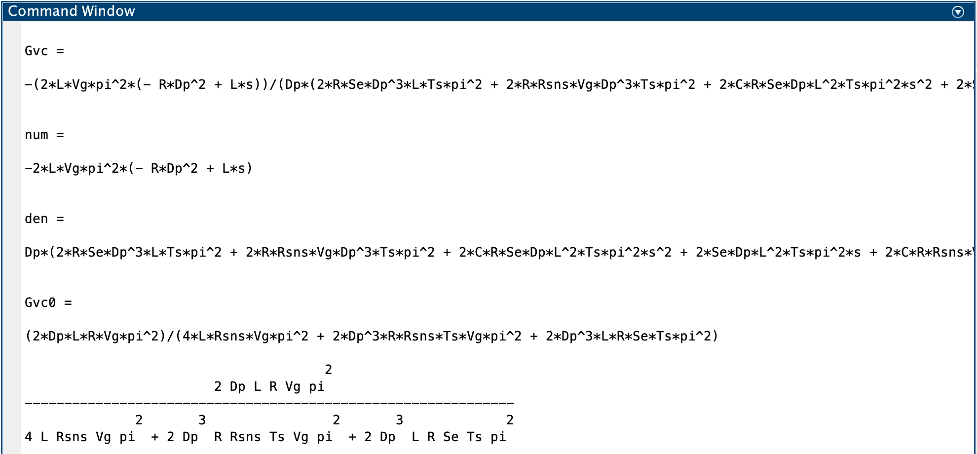
The derived transfer function is as shown in Fig. 3, where we need to do the simplification so that we can get a simplified equation which we guide us to design the control loop and compensator.

Fig. 3Gvc derived results from Matlab

Here, let us assume the following condition for the boost converter:

• Vin = 3.8V
• Vout = 20V
• Dp = Vin/Vout = 0.19
• D = 1-Dp = 0.81
• R = 20Ω
• L = 1µH
• C = 10µF (derated)
• fsw = 3MHz
• Rsns = 0.3Ω
• Se tracks inductor current down-slope

The above parameters will help us on the following equation simplifications.

Simplification - DC gain of G_vc

Here, we are going to use wxMaxima to do the simplification as shown in Fig. 4.

Fig. 4Gvc0 DC gain simplification in wxMaxima

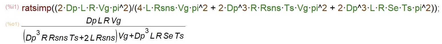
To further simplify the Math equation shown in Fig. 4, we need to plug in the circuit conditions we just defined in the above section by using the following Matlab script.

clc; clear; close all;

Vg=3.8; V=20; R=20; L=1e-6; C=10e-6;
fsw=3e6;
Rsns=0.3;

Dp = Vg/V; D = 1-Dp;
Ts = 1/fsw;

Se = (V-Vg)/L*Rsns;

term1 = Dp^3*R*Rsns*Ts*Vg;
term2 = 2*L*Rsns*Vg;
term3 = Dp^3*L*R*Se*Ts;

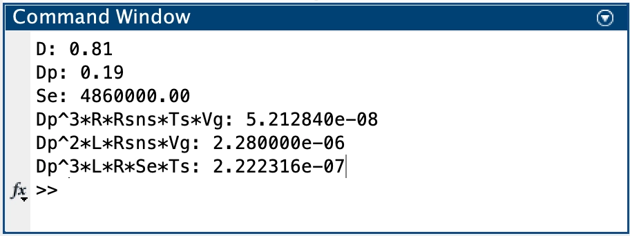
fprintf("\nD: %.2f", D);
fprintf("\nDp: %.2f", Dp);
fprintf("\nSe: %.2f", Se);
fprintf("\nDp^3*R*Rsns*Ts*Vg: %s", term1);
fprintf("\nDp^2*L*Rsns*Vg: %s", term2);
fprintf("\nDp^3*L*R*Se*Ts: %s\n", term3);

Matlab analysis result is as shown in Fig. 5.

Fig. 5Gvc DC gain term analysis from Matlab

Based on the Matlab result, we can set several terms in the denominator to be zero as shown in Fig. 6.

Fig. 6Gvc DC gain term simplification in wxMaxima

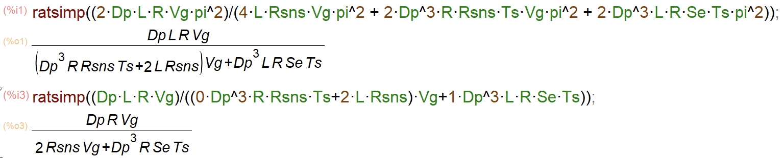
From Fig. 6, we have:

We can get some insights from Eq. 3:

• Higher current sense gain R_sns would result a lower DC gain of G_vc. We can understand it in this way. When we have a perturbation on the VEA voltage, the sensed inductor current will follow due to the closed loop nature. Basically, the product (i_L*R_sns) remains constant. The higher the R_sns, the smaller i_L perturbation will be. Smaller i_L perturbation would result a smaller V_out change on the output voltage.

• Increasing the compensation ramp S_e will decrease the DC gain. Basically, when we have a higher and higher S_e, the control loop is going to behave more and more like a voltage mode controller. For the same amount of perturbation on VEA, the perturbation on the duty cycle is much smaller and as a result a smaller V_out change on the output voltage.

RHP zero

From Fig. 3, we can easily tell the RHPz (right half plane zero) to be:

RHPz is present for any converter if the inductor is not directly connected with the Vout capacitor. Basically, whenever Vout has an undershoot, the switching regulator needs to energize the inductor fist. During this time, the Vout will keep decreasing and that is the fundamental reason why RHPz is present.

Dominant pole

It is going to take a lot of effort to derive the dominant pole and the subharmonic oscillation pole. From Matlab we have:

• den = Dp(2RSeDp^3LTspi^2 + 2RRsnsVgDp^3Tspi^2 + 2CRSeDpL^2Tspi^2s^2 + 2SeDpL^2Tspi^2s + 2CRRsnsVgDpLTspi^2s^2 + 2RsnsVgDpLTspi^2s + 2CRRsnsVgLTs^2s^3 + 4RsnsVgLTs^2s^2 - CRRsnsVgLTspi^2s^2 - 2RsnsVgLTspi^2s + 2CRRsnsVgLpi^2s + 4RsnsVgL*pi^2)

From the above equation, we notice that it is a third-order system. Let us assume that we have one dominant pole and two complexed poles. Therefore, the denominator can be written as:

Eq. 5 can be re-written as:

Here we assume:

Therefore, Eq. 6 can be simplified as:

The denominator result we got from Matlab can be written in the following form:

The following Matlab script is used to plug in the parameter and check which term can be ignored.

clc; clear; close all;

Vg=3.8; V=20; R=20; L=1e-6; C=10e-6;
fsw=3e6;
Rsns=0.3;

Dp = Vg/V; D = 1-Dp;
Ts = 1/fsw;

Se = (V-Vg)/L*Rsns;

term1 = (Dp-1)*L*Rsns*Ts*Vg;
term2 = C*L*R*Rsns*Vg;
term3 = Dp*L^2*Se*Ts;

term4 = Dp^3*R*Rsns*Ts*Vg;
term5 = 2*L*Rsns*Vg;
term6 = Dp^3*L*R*Se*Ts;


fprintf("\n(Dp-1)*L*Rsns*Ts*Vg: %s", term1);
fprintf("\nC*L*R*Rsns*Vg: %s", term2);
fprintf("\nDp*L^2*Se*Ts: %s", term3);
fprintf("\n--------------------");
fprintf("\nDp^3*R*Rsns*Ts*Vg: %s", term4);
fprintf("\n2*L*Rsns*Vg: %s", term5);
fprintf("\nDp^3*L*R*Se*Ts: %s\n", term6);

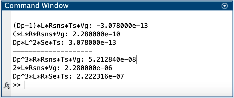
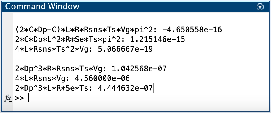
The calculated result from Matlab is as shown in Fig. 7.

Fig. 7d1 terms calculated result from Matlab

Then we can use wxMaxima for simplification. Eventually, the simplified result for d₁ is as shown in Fig. 8.

Fig. 8d1 simplified result from wxMaxima

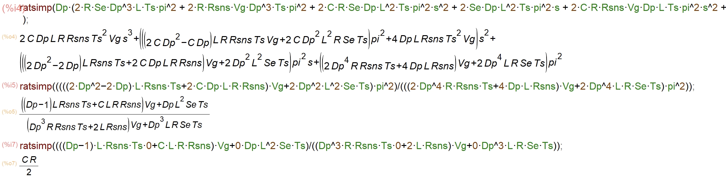
From Fig. 8, we have:

Next, let us try to simplify the term d₂. The Matlab script is as shown below.

clc; clear; close all;

Vg=3.8; V=20; R=20; L=1e-6; C=10e-6;
fsw=3e6;
Rsns=0.3;

Dp = Vg/V; D = 1-Dp;
Ts = 1/fsw;

Se = (V-Vg)/L*Rsns;

term1 = (2*C*Dp-C)*L*R*Rsns*Ts*Vg*pi^2;
term2 = 2*C*Dp*L^2*R*Se*Ts*pi^2;
term3 = 4*L*Rsns*Ts^2*Vg;

term4 = 2*Dp^3*R*Rsns*Ts*Vg;
term5 = 4*L*Rsns*Vg;
term6 = 2*Dp^3*L*R*Se*Ts;


fprintf("\n(2*C*Dp-C)*L*R*Rsns*Ts*Vg*pi^2: %s", term1);
fprintf("\n2*C*Dp*L^2*R*Se*Ts*pi^2: %s", term2);
fprintf("\n4*L*Rsns*Ts^2*Vg: %s", term3);
fprintf("\n--------------------");
fprintf("\n2*Dp^3*R*Rsns*Ts*Vg: %s", term4);
fprintf("\n4*L*Rsns*Vg: %s", term5);
fprintf("\n2*Dp^3*L*R*Se*Ts: %s\n", term6);

The calculated d₂ terms from Matlab are as shown in Fig. 9.

Fig. 9d2 terms calculated result from Matlab

The simplified d₂ result by wxMaxima is as shown in Fig. 10.

Fig. 10d2 simplified result in wxMaxima

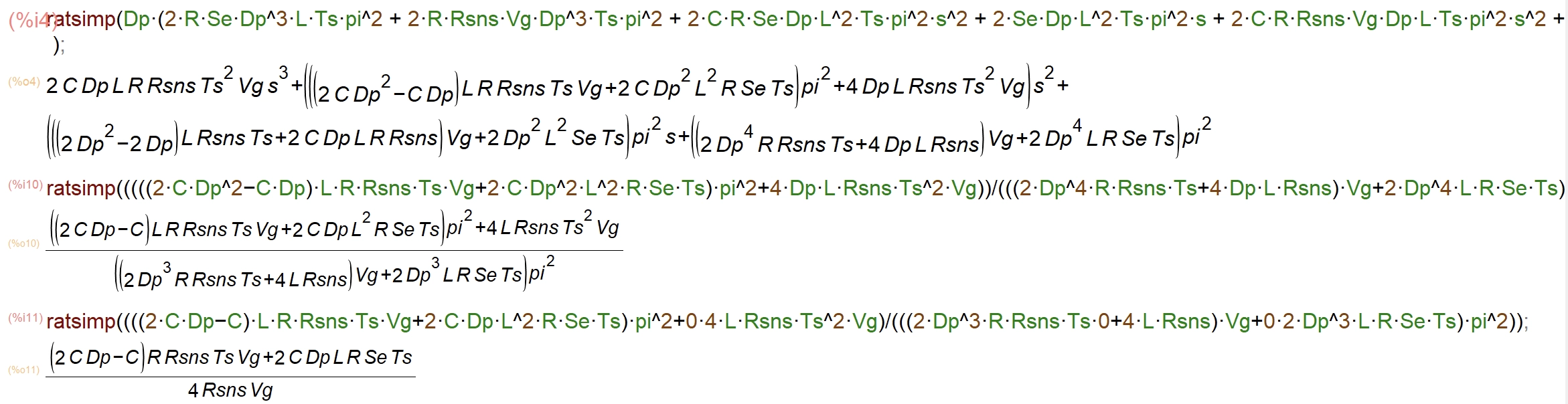
From Fig. 10, we have:

Eq. 11 can be re-written as:

We know that:

Therefore, by combing Eq. 12~13, we have:

let us try to simplify the term d₃. The Matlab script is as shown below.

clc; clear; close all;

Vg=3.8; V=20; R=20; L=1e-6; C=10e-6;
fsw=3e6;
Rsns=0.3;

Dp = Vg/V; D = 1-Dp;
Ts = 1/fsw;

Se = (V-Vg)/L*Rsns;

term4 = Dp^3*R*Rsns*Ts*Vg;
term5 = 2*L*Rsns*Vg;
term6 = Dp^3*L*R*Se*Ts;


fprintf("\nDp^3*R*Rsns*Ts*Vg: %s", term4);
fprintf("\n2*L*Rsns*Vg: %s", term5);
fprintf("\nDp^3*L*R*Se*Ts: %s\n", term6);

The calculated d₂ terms are as shown in Fig. 11.

Fig. 11d3 terms calculated result from Matlab

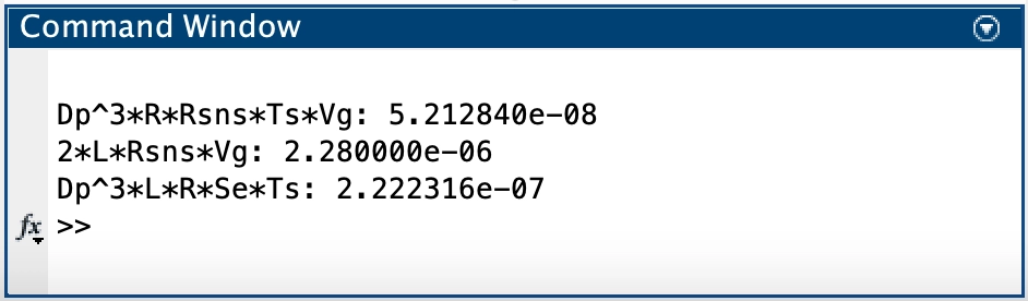
The simplified d₂ result by wxMaxima is as shown in Fig. 12.

Fig. 12d3 simplified result in wxMaxima

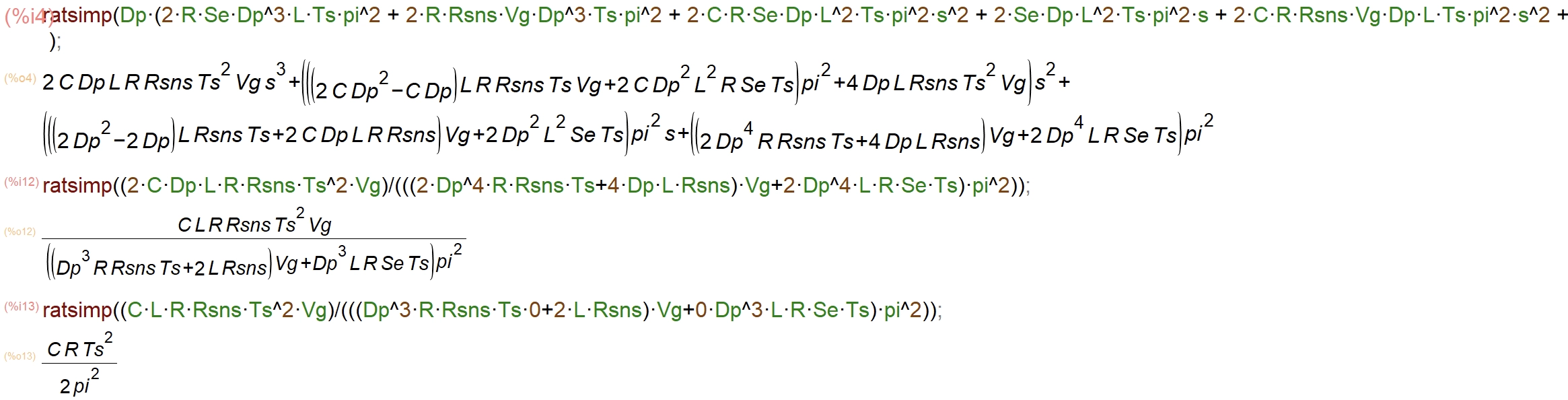
From Fig. 12, we have:

By comparing Eq. 8~9, we have:

Then, we can plug in Eq. 10 into Eq. 16, the dominant pole frequency can be calculated as:

Again, by comparing Eq. 8~9, we have:

Then, we can plug in Eq. 15 into Eq. 18, the subharmonic oscillation pole frequency can be calculated as:

As the name indicated, the subharmonic oscillation pole is located at half of the switching frequency, which is exactly as we expected.

Again, by comparing Eq. 8~9, we have:

Then, we can plug in Eq. 14 and Eq. 17~18 into Eq. 20, the qualifty factor can be calculated as:

Eq. 19 can be simplified as:

Eq. 20 successfully predicts the subhamonic oscillation behavior of the current mode controller. For example, if we do not have the compensation ramp, S_e be equal to 0. Then at 50% duty cycle, quality factor Q will become infinity and subhamonic oscillation will happen.

Peak current mode controlled Boost converter G_vc transfer function

Where, the DC gain is:

The dominant pole is:

The subhamonic oscillation pole is:

The quality factor Q is:

The right half plane zero is:

References and downloads

[1] A New Small-Signal Model for Current-Mode Control - page 24

[2] Gvd derivation of Boost converter - Voltage Mode

[3] He(s) derivation for peak current mode control