POP and AC simulation in Simplis

Ideal transfer function

In Ref. [1], we have derived the G_vd for the Buck converter, which can be written as:

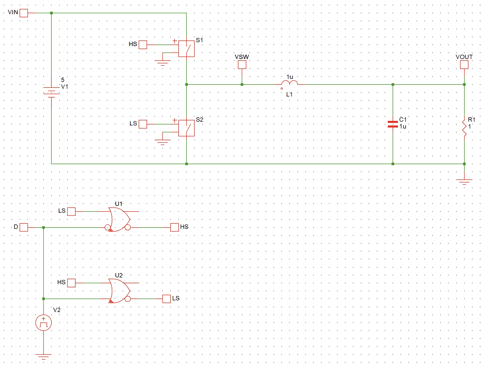
In Ref. [2], we have created the open loop Buck converter model in Simplis as shown in Fig. 1.

Fig. 1Open loop Buck converter model in Simplis^[2]

Next, we can use the following Matlab script to plot the G_vd transfer function^[3].

clc; clear; close all;

L = 1e-6;
C = 1e-6;
R = 1;
Vg = 5;

s = tf('s');

Gvd = Vg/(1+s*L/R+L*C*s^2);

h = bodeplot(Gvd);                    % Plot the Bode plot of G(s)
setoptions(h, 'FreqUnits', 'Hz');   % change frequency scale from rad/sec to Hz
set(findall(gcf,'type','line'),'linewidth',2)
grid on;

The Matlab Bode plot is as shown in Fig. 2.

Fig. 2Open loop Buck converter Gvd bode plot in Matlab

The DC gain is 14dB, which is:

Eq. 2 matches with the math derivation from Eq. 1.

Simplis model

To plot the G_vd transfer function in Simplis, we need to modify the open loop Buck converter model in Ref. [2] as shown in Fig. 3.

Fig. 3Modified open loop Buck converter model in Simplis

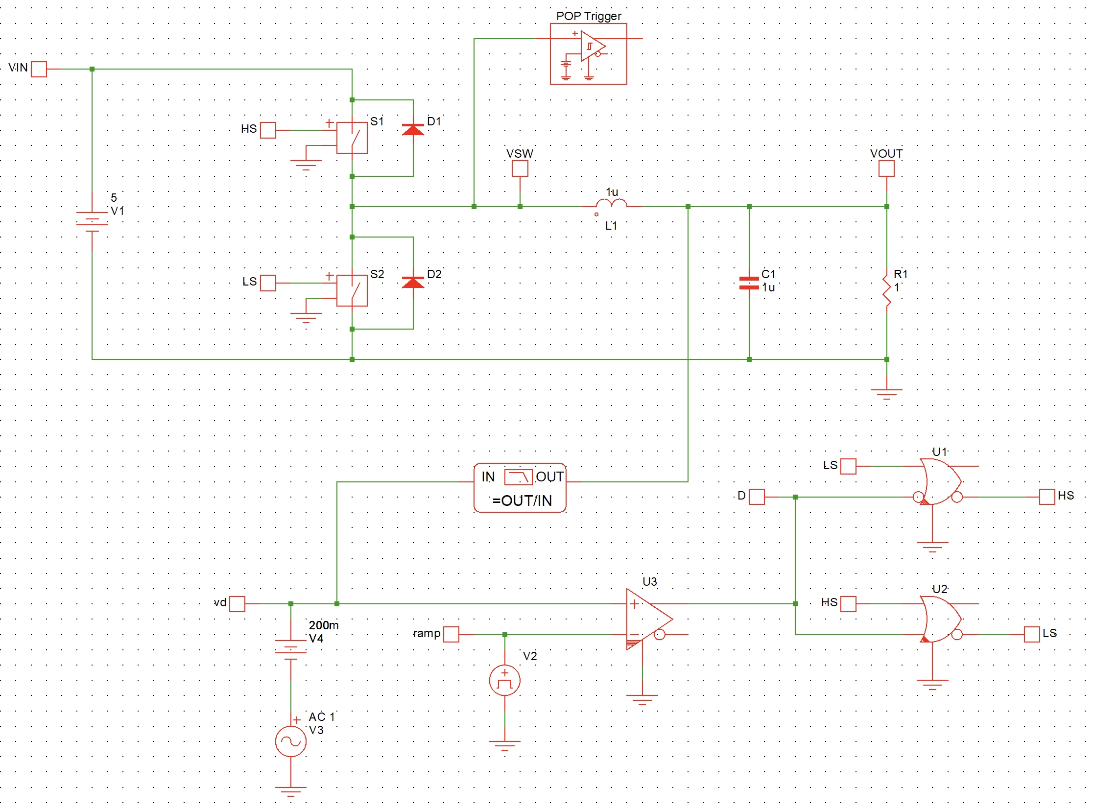
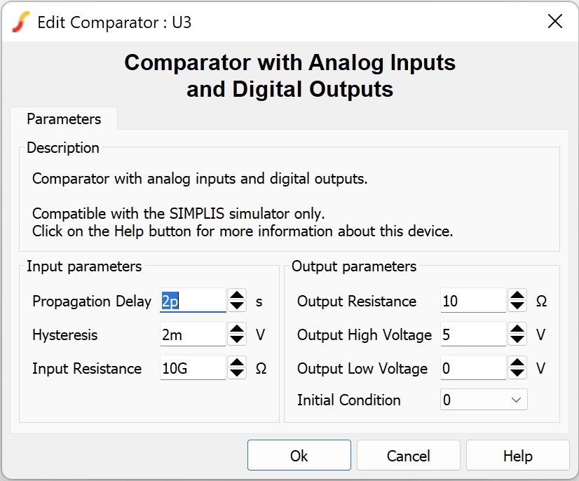
• First, we notice that the waveform generator previously used in Ref. [2] has been changed to a combination of comparator + ramp + DC voltage source. This modification is done so that we can put an AC voltage source in series with the DC voltage source for G_vd AC simulation.

• The property of the comparator is as shown in Fig. 4. Here we change the comparator's input resistance to be 10G.

Fig. 4Comparator properties

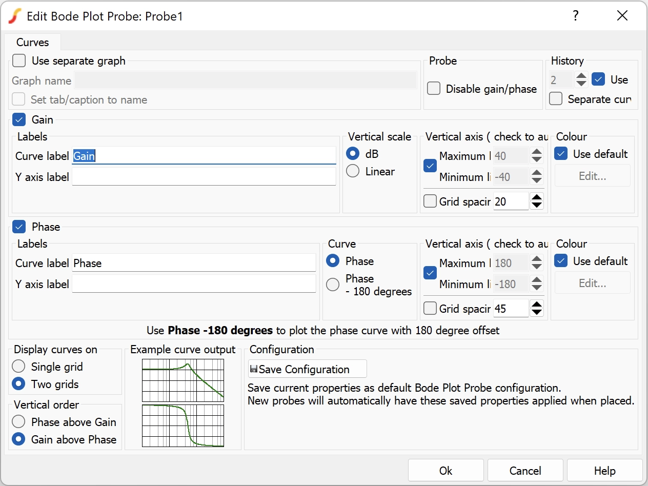
• The property of the Bode plot block is as shown in Fig. 5. I like the way that Gain above Phase. But it is up to you which style you prefer.

Fig. 5Bode plot properties

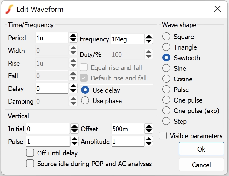
• The property of the waveform generator block is as shown in Fig. 6. Here we choose the Sawtooth option so that after comparing with the 200mV DC voltage source, a square wave can be generated with 20% duty cycle.

Fig. 6Waveform generator properties

• Then, in the Simulator => Choose Analysis..., we can set up the POP analysis as shown in Fig. 7.

Fig. 7POP analysis settings

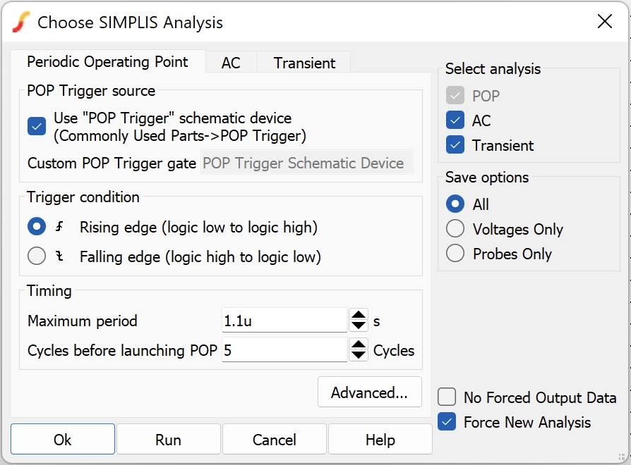
Since the switching frequency is set to be 1MHz, we set the Maximum period to be:

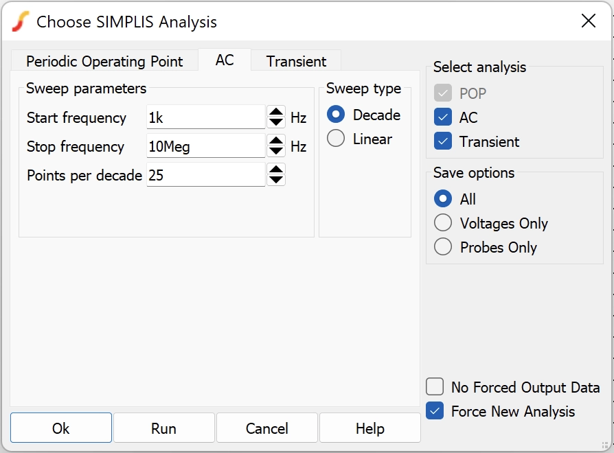
• Next, we can set up the AC analysis properties as shown in Fig. 8.

Fig. 8AC analysis settings

Simulation results

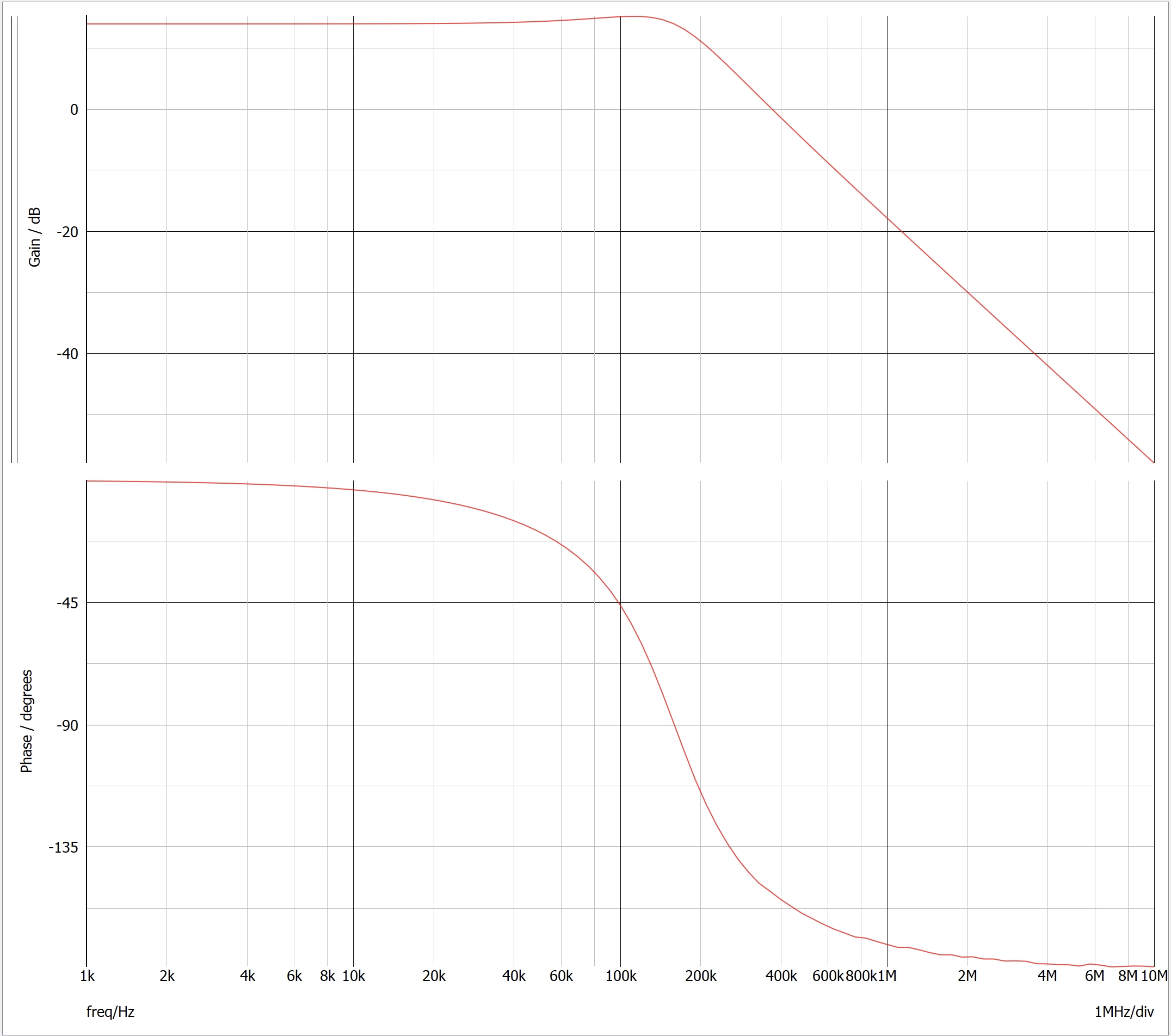
Click the Run button and the AC simulation results will be automatically plotted in Simplis. Since the Bode plot block input is vd while the output is connected to VOUT, the AC simulation results will be G_vd transfer function.

Fig. 9Gvd Bode plot in AC analysis

Compare the results between Simplis and Matlab

Next, we can export the Simplis data out, use Matlab to plot it and compare the results.

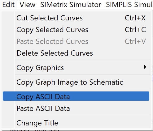
• First, in Simplis, go to Edit => Copy ASCII Data.

Fig. 10Copy simulation data

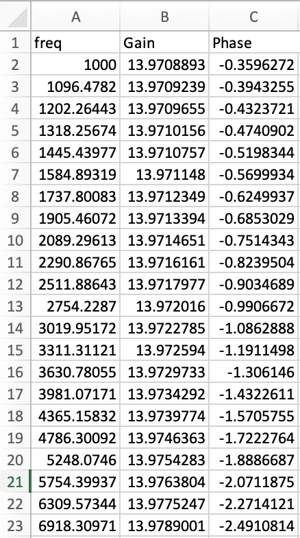
• Next, create a csv file and copy the gain and phase data into the csv file as shown in Fig. 11.

Fig. 11Copy simulation data into CSV file

• Then, let us plot the csv data with s domain bode plot together to compare the results by using the following Matlab script.

clc; clear; close all;

L = 1e-6;
C = 1e-6;
R = 1;
Vg = 5;

s = tf('s');

Gvd = Vg/(1+s*L/R+L*C*s^2);

h = bodeplot(Gvd);                    % Plot the Bode plot of G(s)
setoptions(h, 'FreqUnits', 'Hz');   % change frequency scale from rad/sec to Hz
set(findall(gcf,'type','line'),'linewidth',2)
grid on;
hold on;

% read simplis simulation results from csv file
data = csvread("simplis.csv", 1, 0);
freq = data(:,1);
mag = data(:,2);
phase = data(:,3);

ax = findobj(gcf, 'type', 'axes');
phase_ax = ax(1);
mag_ax = ax(2);


% append simplis plot to bode plot
plot(phase_ax, freq, phase, 'r--', 'LineWidth', 2);
plot(mag_ax, freq, mag, 'r--', 'LineWidth', 2);
legend('Math', 'Simplis')

The Matlab plot is as shown in Fig. 12.

Fig. 12Bode plot comparision between Mathematics and Simplis

References and materials

[1] Power stage transfer function derivations

[2] Open loop Buck converter in Simplis

[3] Write transfer function in Matlab for bode plot

[4] buck.m - download

[5] simplis.csv - download